Tutorial 12: Image segmentation and object detection using the radiation camera

In this tutorial, we will use the radiation model to render a synthetic scene containing multiple objects, then generate image segmentation masks and bounding boxes for computer vision and machine learning applications. This tutorial demonstrates how Helios can be used to create annotated synthetic datasets for training object detection models.

We will create a scene with Stanford Bunny and Dragon models, render them using the radiation camera with RGB bands, and export the results in COCO JSON format for use with popular machine learning frameworks.

Overview

This tutorial covers the following topics:

1. Loading and positioning multiple 3D models in a scene
2. Setting up spectral properties using color references
3. Configuring a radiation camera for RGB imaging
4. Adding object labels for segmentation
5. Running the radiation model to render the scene
6. Exporting segmentation masks and bounding boxes in COCO format
7. Visualizing the results

The main output of this tutorial will be:

• A rendered RGB image of the scene
• COCO-format JSON file with segmentation masks and bounding boxes
• Python visualization script to view the results

1. Creating the Scene Geometry

We begin by loading several 3D models to create an interesting scene for object detection:

#include "RadiationModel.h"
#include "Visualizer.h"
 
using namespace helios;
 
int main(){
 
    Context context;
 
    // Load two Stanford Bunny models and position them
    std::vector<uint> UUIDs_bunny_1 = context.loadPLY( "../../../PLY/StanfordBunny.ply" );
    context.translatePrimitive( UUIDs_bunny_1, make_vec3(0.15,0,0));
 
    std::vector<uint> UUIDs_bunny_2 = context.loadPLY( "../../../PLY/StanfordBunny.ply" );
    context.translatePrimitive( UUIDs_bunny_2, make_vec3(-0.15,0,0));
 
    // Load and scale the Stanford Dragon model
    std::vector<uint> UUIDs_dragon = context.loadPLY( "../../../PLY/StanfordDragon.ply", make_vec3(0.025,0,0), 0.2, nullrotation );
 
    // Add a ground plane
    std::vector<uint> UUIDs_tile = context.addTile( nullorigin, make_vec2(1,1), nullrotation, make_int2(1000,1000));
    context.setPrimitiveData(UUIDs_tile, "twosided_flag", 0u);

In this section, we load three distinct objects: two bunny models positioned at different locations, and a dragon model that is scaled down and positioned at the origin. The ground plane provides a base for the scene and helps with realistic lighting.

2. Setting Material Properties

Next, we assign realistic colors and material properties to our objects using the Calibrite color reference standards:

// Load color reference data
context.loadXML( "plugins/radiation/spectral_data/color_board/Calibrite_ColorChecker_Classic_colorboard.xml", true);
 
// Assign colors to each object
context.setPrimitiveData(UUIDs_bunny_1, "reflectivity_spectrum", "ColorReference_Calibrite_15"); //red
context.setPrimitiveData(UUIDs_bunny_2, "reflectivity_spectrum", "ColorReference_Calibrite_04"); //green  
context.setPrimitiveData(UUIDs_dragon, "reflectivity_spectrum", "ColorReference_Calibrite_10"); //purple
context.setPrimitiveData( UUIDs_tile, "reflectivity_spectrum", "ColorReference_Calibrite_13"); //dark blue
 
// Set specular properties for realistic shading
context.setPrimitiveData( UUIDs_bunny_1, "specular_exponent", 10.f);
context.setPrimitiveData( UUIDs_bunny_2, "specular_exponent", 10.f);
context.setPrimitiveData( UUIDs_dragon, "specular_exponent", 10.f);

The Calibrite color board provides spectrally accurate color references that ensure realistic material appearance. The specular exponent controls how shiny the surfaces appear.

3. Adding Object Labels for Segmentation

For machine learning applications, we need to label each object so we can generate segmentation masks. We assign unique labels to identify different object types:

// Set up object labels for segmentation
// First bunny gets ID 0 with label "bunny"  
context.setPrimitiveData(UUIDs_bunny_1, "bunny", 0u);
 
// Second bunny gets ID 8 with label "bunny" (ID value doesn't matter, only consistency within object)
context.setPrimitiveData(UUIDs_bunny_2, "bunny", 8u);
 
// Dragon gets a different class label "dragon"
context.setPrimitiveData(UUIDs_dragon, "dragon", 6u);

The key insight here is that all primitives belonging to the same object instance must have the same ID value, but the actual ID value doesn't matter. What matters is the label name ("bunny" vs "dragon") for distinguishing different object classes.

4. Setting Up the Radiation Model

Now we configure the radiation model with RGB bands and lighting:

// Initialize radiation model
RadiationModel radiation(&context);
 
// Add color calibration target (optional)
CameraCalibration calibration(&context);
calibration.addCalibriteColorboard( make_vec3(0,0.23,0.001), 0.025 );
 
// Set up sun lighting
SphericalCoord sun_dir = make_SphericalCoord(deg2rad(45), -deg2rad(45));
uint sunID = radiation.addSunSphereRadiationSource(sun_dir );
radiation.setSourceSpectrum( sunID, "solar_spectrum_ASTMG173");
 
// Create RGB radiation bands
radiation.addRadiationBand("red");
radiation.disableEmission("red");
radiation.setDiffuseRadiationExtinctionCoeff( "red", 0.2f, sun_dir);
radiation.setScatteringDepth("red", 3);
 
radiation.copyRadiationBand("red", "green");
radiation.copyRadiationBand("red", "blue");
 
std::vector<std::string> bandlabels = {"red", "green", "blue"};
radiation.setDiffuseSpectrum( bandlabels, "solar_spectrum_ASTMG173");

We create three radiation bands (red, green, blue) with identical scattering properties. The sun is positioned at a 45-degree elevation and azimuth angle to provide good lighting of the objects.

5. Camera Setup

The radiation camera captures our synthetic scene. We configure it with appropriate resolution and field of view:

std::string cameralabel = "bunnycam";
 
// Configure camera parameters
vec3 camera_position = make_vec3(-0.01, 0.05, 0.6f);
vec3 camera_lookat = make_vec3(0, 0.05, 0);
CameraProperties cameraproperties;
cameraproperties.camera_resolution = make_int2(1024, 1024);
cameraproperties.focal_plane_distance = 0.5;
cameraproperties.lens_diameter = 0.002f;
cameraproperties.FOV_aspect_ratio = 1;
cameraproperties.HFOV = 50.f;
 
// Add the camera to the radiation model
radiation.addRadiationCamera(cameralabel, bandlabels, camera_position, camera_lookat, cameraproperties, 100);
 
// Set camera spectral response to simulate iPhone camera
context.loadXML( "plugins/radiation/spectral_data/camera_spectral_library.xml", true);
radiation.setCameraSpectralResponse(cameralabel, "red", "iPhone12ProMAX_red");
radiation.setCameraSpectralResponse(cameralabel, "green","iPhone12ProMAX_green");
radiation.setCameraSpectralResponse(cameralabel, "blue", "iPhone12ProMAX_blue");

The camera is positioned to capture all objects in the scene. We use iPhone spectral response curves to simulate realistic color capture.

6. Rendering and Export

Finally, we run the radiation model and export the results:

// Update geometry and run radiation calculation
radiation.updateGeometry();
radiation.runBand( bandlabels);
 
// Process the image using standard pipeline
radiation.applyImageProcessingPipeline("bunnycam", "red", "green", "blue", 1, 1, 1, 1);
 
// Save the rendered RGB image
std::string image_file = radiation.writeCameraImage( cameralabel, bandlabels, "RGB", "../output/");
 
// Export bounding boxes and segmentation masks in COCO format
radiation.writeImageBoundingBoxes( cameralabel, {"bunny","dragon"}, {0, 1}, image_file, "classes.txt", "../output/");
radiation.writeImageSegmentationMasks( cameralabel, {"bunny","dragon"}, {0, 1}, "../output/bunnycam_segmentation.json", image_file );
 
// Initialize visualizer
Visualizer vis(1000);
vis.displayImage("../output/bunnycam_RGB.jpeg");
 
// Auto-calibrate camera image using colorboard reference values with quality report
std::string corrected_image = radiation.autoCalibrateCameraImage("bunnycam", "red", "green", "blue", "../output/auto_calibrated_bunnycam.jpeg", true);

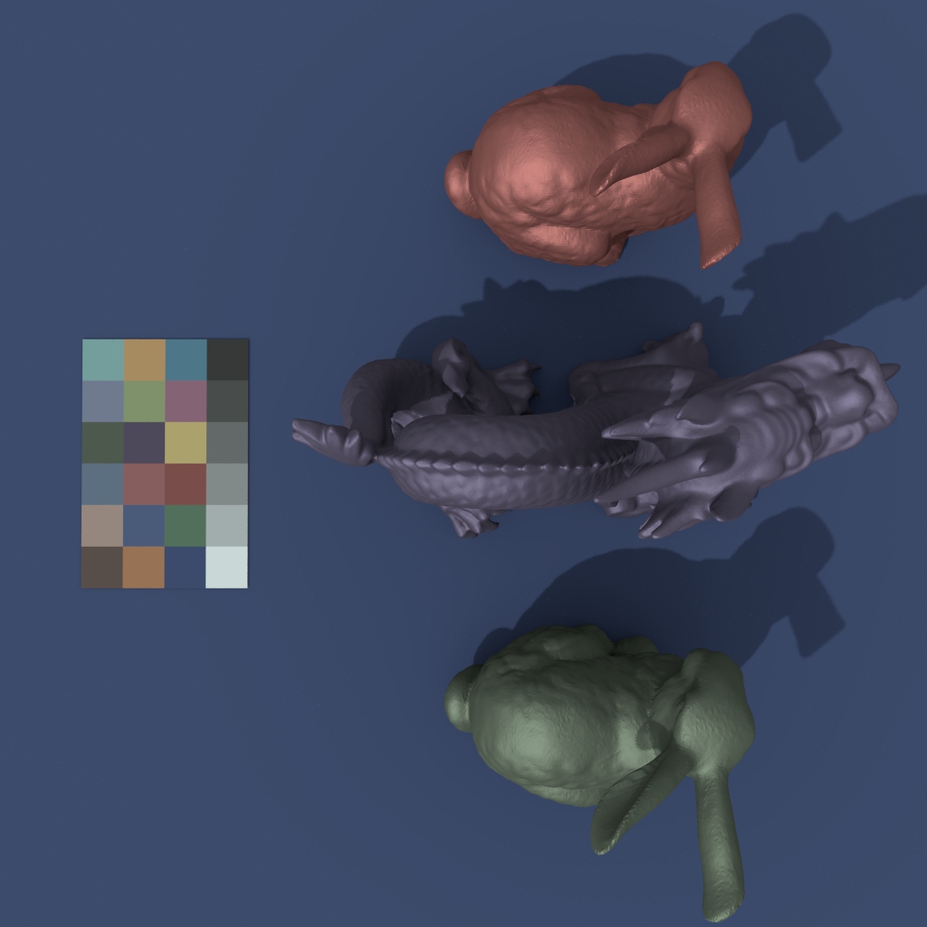
Rendered RGB Image of the Scene

The writeImageBoundingBoxes() and writeImageSegmentationMasks() functions export the object detection data in COCO JSON format, which is compatible with popular machine learning frameworks like detectron2, YOLO, and others.

The autoCalibrateCameraImage() function performs automatic color calibration using the colorboard reference values we added earlier. This step corrects for any color biases in the simulated camera and produces a more color-accurate image. The true parameter enables a detailed quality report that shows the calibration accuracy.

7. Understanding the Output

This tutorial generates several important output files:

• bunnycam_RGB.jpeg: The rendered RGB image of the scene
• auto_calibrated_bunnycam.jpeg: Color-calibrated version of the RGB image using colorboard reference values
• bunnycam_boundingboxes.json: COCO-format bounding boxes around detected objects
• bunnycam_segmentation.json: COCO-format segmentation masks for each object
• classes.txt: Text file mapping class IDs to class names

The COCO JSON format includes:

• Image metadata (dimensions, file path)
• Category definitions (class names and IDs)
• Annotation data (segmentation polygons, bounding boxes, areas, object IDs)

8. Python Visualization

The tutorial includes a Python script (visualize_segmentation.py) to visualize the segmentation results:

python3 visualize_segmentation.py --json output/bunnycam_segmentation.json

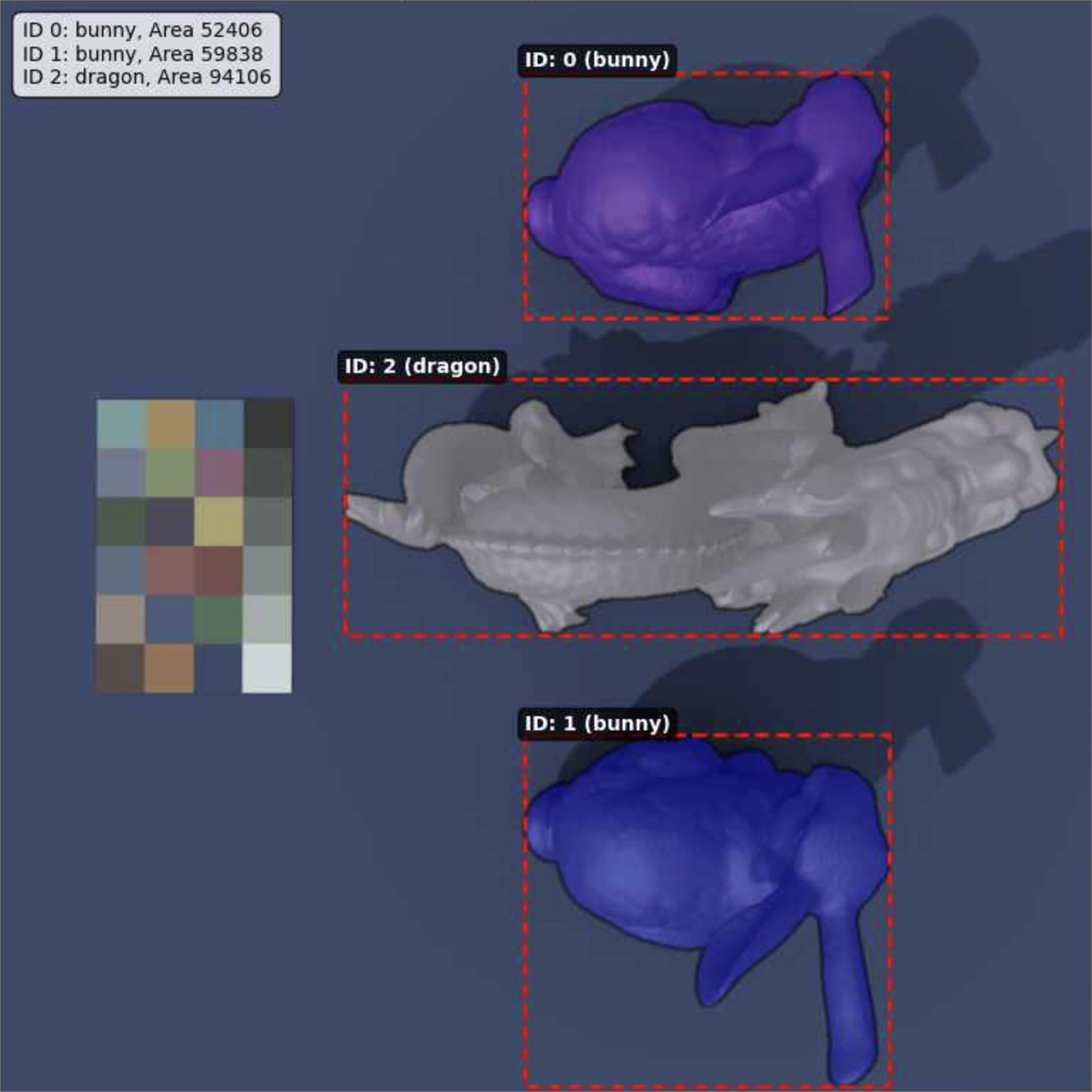
RGB image with segmentation masks

This script displays the original image alongside the same image with segmentation masks and bounding boxes overlayed, making it easy to verify the quality of the synthetic annotations.

9. Applications

This tutorial demonstrates techniques useful for:

• Synthetic dataset generation: Create large labeled datasets for training object detection models
• Domain transfer: Generate synthetic data to supplement real-world training data
• Algorithm testing: Test computer vision algorithms on controlled synthetic scenes
• Rare scenario simulation: Generate difficult or dangerous scenarios that are hard to capture in reality

Complete Code

The complete code for this tutorial can be found in samples/tutorial12/main.cpp, along with the Python visualization script in samples/tutorial12/visualize_segmentation.py.