System Requirements

Dependencies	NVIDIA CUDA 9.0+
Platforms	Windows, Linux
GPU	Required - NVIDIA CUDA-capable GPU

Quick Start

from pyhelios import Context, EnergyBalanceModel
from pyhelios.types import vec3, vec2
 
with Context() as context:
    # Create minimal geometry
    uuid = context.addPatch(center=vec3(0, 0, 1), size=vec2(1, 1))
 
    # Set required primitive data
    context.setPrimitiveData(uuid, "air_temperature", 300.0)  # Kelvin
 
    # Use energy balance plugin
    with EnergyBalanceModel(context) as energybalance:
        # Add radiation bands
        energybalance.addRadiationBand("PAR")
        energybalance.addRadiationBand("NIR")
        energybalance.addRadiationBand("LW")
 
        # Run steady-state model
        energybalance.run()
 
        # Get results
        temperature = context.getPrimitiveData(uuid, "temperature")
        print(f"Surface temperature: {temperature[0]:.2f} K")

Additional Dependencies

Package
NVIDIA CUDA 9.0+	Mac OSX: Not available	Use CUDA installer	Use CUDA installer

For detailed CUDA installation instructions, see the comprehensive CUDA Setup Guide, which covers:

Choosing the correct CUDA toolkit version: Choosing the Right CUDA Version
Platform-specific installation steps (Windows, Linux)
GPU timeout settings for Windows: Windows-Specific: GPU Timeout Settings
OptiX requirements: OptiX Requirements (Radiation Plugin Only)
Troubleshooting common issues

Known Issues

None.

Introduction

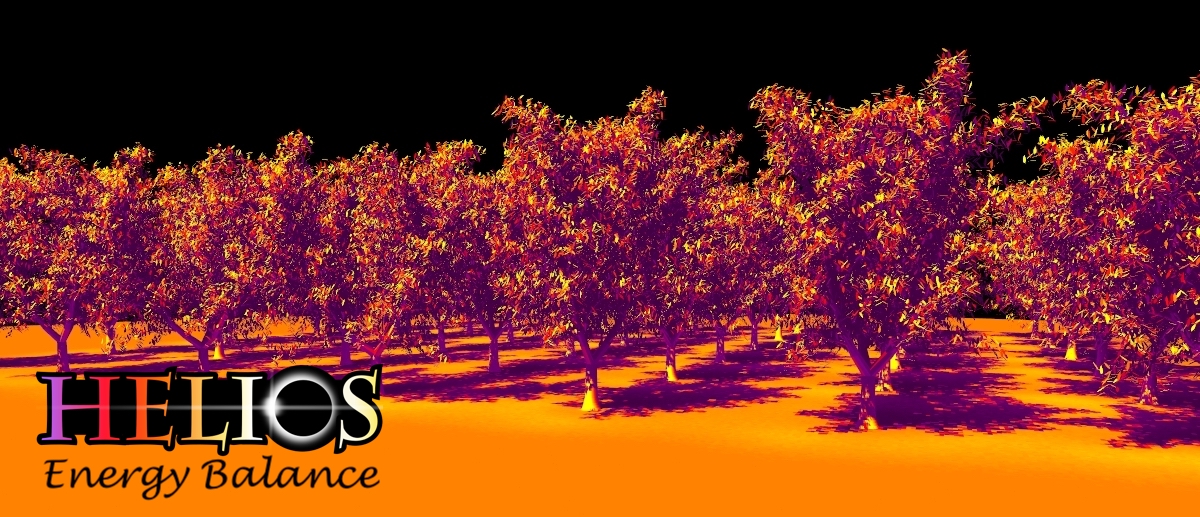
This model plugin calculates a local energy balance for every primitive, and ultimately predicts sensible, latent, and longwave fluxes as well as surface temperature. The energy balance equation is solved in parallel on the GPU to accelerate calculations.

The model is solving the steady-state budget between absorbed radiation, emitted radiation, sensible heat exchange, and latent heat exchange, which is written as

\[ R-n_s\varepsilon\sigma T_s^4 = c_p g_H \left( T_s-T_a \right) + \lambda g_M \left(\frac{e_s(T_s)f_s-e_s(T_a)h}{p_{atm}}\right)+C_p\frac{dT_s}{dt}+Q_{other}\]

Variables in this equation are listed in this table:

Variable (units)	Description
\(R\) (W/m²)	Absorbed all-wave radiation flux (shortwave+longwave).
\(T_s\) (K)	Primitive surface temperature.
\(T_a\) (K)	Air temperature just outside primitive boundary-layer.
\(g_H\) (mol air/m²-s)	Conductance to heat from primitive surface to outside of boundary-layer.
\(g_S\) (mol air/m²-s)	Conductance to moisture between sub-surface air spaces to surface (e.g., for leaves this is stomatal conductance).
\(g_M\) (mol air/m²-s)	Conductance to moisture from primitive surface to outside of boundary-layer.
\(e_s(T)\) (Pa)	Saturation vapor pressure at temperature T. Calculated from Tetens equation (see en.wikipedia.org/wiki/Tetens_equation)
\(f_s\)	Relative humidity of air at primitive surface.
\(h\)	Relative humidity of air outside of boundary-layer.
\(p_{atm}\) (Pa)	Atmospheric pressure.
\(C_p\) (J/m²/^oC)	Heat capacity of object.
\(Q_{other}\) (W/m²)	Any surface fluxes other than radiation, convection, or latent (e.g., storage).
\(n_s\)	Number of primitive faces with heat transfer (e.g., typically \(n_s=1\) for leaves, and \(n_s=0\) for the ground.

Constants are given by:

Constant (units)	Value	Description
\(c_p\) (J/mol/K)	29.25	Heat capacity of air.
\(\lambda\) (J/mol)	44,000	Latent heat of vaporization of air.

Class Constructor

Constructors
EnergyBalanceModel

The EnergyBalanceModel class is initialized by passing the Helios context as an argument to the constructor.

Primitive Data

Input Primitive Data

Primitive Data	Units	Data Type	Description	Available Plug-ins	Default Value
radiation_flux_[*]	W/m²	float	Net absorbed radiation flux for band [*] (e.g., radiation_flux_PAR).	Can be computed by RadiationModel plug-in.	N/A (must add at least one band)
wind_speed	m/s	float	Air wind speed just outside of primitive boundary-layer.	N/A	1 m/s
object_length	m	float	Characteristic dimension of object formed by primitive.	N/A	Square root of primitive surface area
boundarylayer_conductance	mol air/m²-s	float	Leaf boundary-layer conductance to heat.	BoundaryLayerConductanceModel plug-in	Try calculating from model \(0.135\sqrt{\frac{U}{L}}\)
air_temperature	Kelvin	float	Ambient air temperature outside of surface boundary layer.	N/A	300 K
moisture_conductance	mol air/m²-s	float	Conductance to moisture between sub-surface air spaces and surface (e.g., for leaves this is stomatal conductance).	Can be computed by StomatalConductanceModel plug-in.	0
surface_humidity	unitless	float	Relative humidity of air immediately above surface evaporating site.	N/A	1.0 (saturated)
air_humidity	unitless	float	Ambient air relative humidity outside of surface boundary layer.	N/A	0.5
air_pressure	Pascals	float	Atmospheric pressure.	N/A	101,000 Pa
heat_capacity	J/m²/^oC	float	Heat capacity of object.	N/A	0
other_surface_flux	W/m²	float	Other surface energy fluxes.	N/A	0
twosided_flag	N/A	uint	Flag indicating the number of primitive faces with heat transfer (twosided_flag = 0 for one-sided heat transfer; twosided_flag = 1 for two-sided heat transfer). Can also be set via the material system using Context::setMaterialTwosidedFlag(). When a user-assigned material exists, the material's twosided_flag takes precedence over primitive data.	N/A	1
stomatal_sidedness	\(\zeta\)	float	Ratio of stomatal density on the upper leaf surface to the sum of the stomatal density on upper and lower leaf surfaces. Note: if "twosided_flag" is equal to 0, stomatal_sidedness will be automatically set to 0.	N/A	0

Default Output Primitive Data

Primitive Data	Units	Data Type	Description
temperature	Kelvin	float	Primitive surface temperature.
sensible_flux	W/m²	float	Sensible heat flux.
latent_flux	W/m²	float	Latent heat flux.

Optional Output Primitive Data

Primitive Data	Units	Data Type	Description
boundarylayer_conductance_out	mol air/m²-s	float	Primitive boundary-layer conductance calculated by this plug-in.
vapor_pressure_deficit	mol/mol	float	Surface vapor pressure deficit.
storage_flux	W/m²	float	Storage heat flux.
net_radiation_flux	W/m²	float	Primitive net radiation flux (absorption minus emission).

Using the Energy Balance Model Plug-in

Input Variables

Inputs to the model are set by creating primitive variable data in the usual way. If a variable needed for a model input has not been create in the Context, the default value is assumed.

Input Radiative Bands

In order for the model to calculate the absorbed all-wave radiation flux, it needs to know the names of all radiation bands that were added to the radiation model. This is done using the function addRadiationBand(). In the following example, assume we have three radiative wavebands "PAR", "NIR", and "LW".

# Initialize the Model
with EnergyBalanceModel(context) as energybalance:
    energybalance.addRadiationBand("PAR")
    energybalance.addRadiationBand("NIR")
    energybalance.addRadiationBand("LW")

Boundary-layer Conductance Model

The primitive boundary-layer conductance can either be set using the BoundaryLayerConductanceModel plug-in, or using the default model which is the Polhausen equation. Note also that custom conductance values can also be provided by setting the value of primitive data labeled 'boundarylayer_conductance', which overrides the computed model value.

It is also important to note that, by default, the length scale used to calculate the boundary-layer conductance is taken to be the square root of the primitive surface area. If the size of the object is different from the size of the primitive, then it is important to manually set the length scale to be the size of the object, as this is the relevant scale for boundary-layer development.

The default boundary-layer conductance is calculated as

\(g_H = 0.135 n_s\sqrt{\frac{U}{L}}\),

where \(U\) is the wind speed just outside of the primitive boundary-layer, and \(L\) is the characteristic length/dimension of the object that the primitive belongs to. For a leaf consisting of a single primitive, \(L\) could be assumed to be the length of the primitive. \(n_s\) is the number of primitive faces, which is determined by the value of primitive data "twosided_flag" (twosided_flag=0 is single-sided and \(n_s=1\), twosided_flag=1 is two-sided and \(n_s=2\)).

Moisture Conductance

For surfaces that are not completely dry or completely saturated with water, availability of water at the surface determines the rate of moisture transfer from the surface. This is represented by the surface moisture conductance \(g_S\), and corresponds to the conductance between the sub-surface air spaces and the surface.

For a dry surface, \(g_S=0\) and thus there is no moisture transfer at the surface. For a surface that is saturated with water (e.g., a lake, puddle), \(g_S\rightarrow\infty\) as the supply of water at the surface is theoretically infinite.

For surfaces such as leaves and the soil in which surface moisture is present but limited, \(g_S\) will have some intermediate value typically on the order of 0.1 mol air/m²-s.

For leaves, \(g_S\) corresponds to the conductance to water vapor between the intercellular (sub-stomatal) air spaces and the surface of the leaf, which we call the stomatal conductance. When stomata are closed, \(g_S\rightarrow 0\), as water transfer is restricted by the stomata.

For the soil surface, the physical interpretation of \(g_S\) is slightly less intuitive, and corresponds to the rate at which water vapor can diffuse from just below the soil to the surface. This is impacted by the soil texture, and the "tortuosity" of the path water vapor must take through the soil, among other factors.

Once the water vapor has diffused to the surface, the rate of transfer is then determined by the surface boundary-layer conductance. The sub-surface conductance and boundary-layer conductance act in serial, and can be combined to yield an overall moisture conductance between the sub-surface air spaces and the outside of the boundary layer according to

\(g_M = 1.08g_Hg_S\left[\dfrac{\zeta}{1.08g_H+g_S\zeta}+\dfrac{(1-\zeta)}{1.08g_H+g_S(1-\zeta)}\right]\),

where \(g_H\) is the boundary-layer conductance to heat, and \(1.08g_H\) gives the boundary-layer conductance to moisture considering the differences in diffusivity between water vapor and heat.

\(\zeta=\dfrac{D_{upper}}{D_{lower}+D_{upper}}\)

is the stomatal sidedness, which is the ratio of the stomatal density of the upper leaf surface to the sum of the upper and lower leaf surface densities, which is set by the primitive data value "stomatal_sidedness". For leaves, \(\zeta=0\) corresponds to hypostomatous leaves (stomata on one side), and \(\zeta=0.5\) to amphistomatous leaves (stomata equally on both sides). It is important to note that if \(n_s=1\), then the value of \(\zeta\) will be overridden and set to 0.

Running the Steady-State Model

The model is run assuming steady-state conditions (heat storage term is zero) using the run() function, which will run the model for all primitives in the Context if no argument is given, or will run the model for a subset of primitives if a list of UUIDs is given as the argument.

Functions to run the steady-state energy balance model.
Model Run Function	Description
run()	Run the model for all primitives in the Context.
run(uuids)	Run the model for a select set of primitives in the Context, which are specified by a list of their UUIDs.

from pyhelios import Context, EnergyBalanceModel
from pyhelios.types import vec3, vec2
 
# Initialize the Context
with Context() as context:
    # Add Patch primitive
    center = vec3(0, 0, 1)
    size = vec2(1, 1)
    UUID = context.addPatch(center, size)
 
    with EnergyBalanceModel(context) as energybalance:
        energybalance.addRadiationBand("PAR")
        energybalance.addRadiationBand("NIR")
        energybalance.addRadiationBand("LW")
 
        energybalance.run()

Unsteady model with heat storage

Additional functions are available to run the unsteady energy balance model with heat storage. If the timestep argument "dt" is passed with value greater than 0, and the heat capacity \(C_p\) is greater than 0, the unsteady energy balance equation will be applied with the heat storage term included. The following equation is then solved for the surface temperature at time \(t+\Delta t\)

\[ R-n_s\varepsilon\sigma T_s(t+\Delta t)^4 - c_p g_H \left( T_s(t+\Delta t)-T_a \right) - \lambda g_M \left(\frac{e_s(T_s(t+\Delta t))f_s-e_s(T_a)h}{p_{atm}}\right)-Q_{other} + C_p\dfrac{T_s(t+\Delta t) - T_s(t)}{\Delta t}.\]

The timestep should be chosen such that it is significantly smaller than the characteristic time constant of heat storage.

Functions for running the unsteady energy balance model are listed below.

Functions to run the unsteady energy balance model.
Model Run Function	Description
run(dt)	Run the model for all primitives in the Context and advance in time by dt seconds.
run(uuids, dt)	Run the model for a select set of primitives in the Context, which are specified by a list of their UUIDs, and advance in time by dt seconds.

Note that you can run the steady-state model for some primitives but run the unsteady model for others simply by changing the value of the heat capacity primitive data. This is illustrated in the code example below.

from pyhelios import Context, EnergyBalanceModel
from pyhelios.types import vec3, vec2
 
# Initialize the Context
with Context() as context:
    # Add one Patch primitive
    center = vec3(0, 0, 1)
    size = vec2(1, 1)
    UUID1 = context.addPatch(center, size)
 
    # Add a second Patch primitive
    center = vec3(2, 0, 1)
    UUID2 = context.addPatch(center, size)
 
    # Set the heat capacity of the first patch so that the unsteady energy balance model will be run
    Cp = 10000  # J/m^2-oC
    context.setPrimitiveData(UUID1, "heat_capacity", Cp)
 
    with EnergyBalanceModel(context) as energybalance:
        energybalance.addRadiationBand("PAR")
        energybalance.addRadiationBand("NIR")
        energybalance.addRadiationBand("LW")
 
        dt = 180
        energybalance.run(dt)

Dependencies	NVIDIA CUDA 9.0+
Python Import	`from pyhelios import EnergyBalanceModel`
Main Class	EnergyBalanceModel

Table of Contents