System Requirements

Dependencies	None
Platforms	Windows, Linux, macOS
GPU	Not required

Quick Start

from pyhelios import Context, PhotosynthesisModel
from pyhelios.types import vec3, vec2
 
with Context() as context:
    # Create a simple patch
    patch_uuid = context.addPatch(center=vec3(0, 0, 0), size=vec2(0.1, 0.1))
 
    # Set required primitive data
    context.setPrimitiveData(patch_uuid, "radiation_flux_PAR", 500.0)  # W/m²
    context.setPrimitiveData(patch_uuid, "temperature", 298.15)  # K
    context.setPrimitiveData(patch_uuid, "air_CO2", 400.0)  # µmol/mol
    context.setPrimitiveData(patch_uuid, "moisture_conductance", 0.3)  # mol/m²-s
    context.setPrimitiveData(patch_uuid, "boundarylayer_conductance", 1.0)  # mol/m²-s
 
    # Create photosynthesis model
    with PhotosynthesisModel(context) as photo:
        # Use species from library
        photo.setFarquharCoefficientsFromLibrary("Almond")
 
        # Run model
        photo.run()
 
        # Get results
        A = context.getPrimitiveData(patch_uuid, "net_photosynthesis")
        print(f"Net photosynthesis: {A[0]:.2f} µmol CO₂/m²-s")

Class Constructor

Constructors
PhotosynthesisModel

Primitive Data

Input Primitive Data

Primitive Data Label	Symbol	Units	Data Type	Description	Available Plug-ins	Default Value
radiation_flux_PAR	\(Q\)	W/m²	float	Radiative flux in PAR band. NOTE: this is automatically converted to units of photon flux density, which are the units used in the photosynthesis model.	Can be computed by RadiationModel plug-in.	0
temperature	\(T_s\)	Kelvin	float	Primitive surface temperature.	Can be computed by EnergyBalanceModel plug-in.	300 K
air_CO2	\(C_a\)	\(\mu\)mol CO₂/mol air	float	CO₂ concentration of air outside of primitive boundary-layer.	N/A	390 \(\mu\)mol/mol
moisture_conductance	\(g_S\)	mol air/m²-s	float	Conductance to moisture between sub-stomatal cells and leaf surface (i.e., stomatal conductance).	Can be computed by StomatalConductanceModel plug-in.	0.25 mol/m²-s
boundarylayer_conductance**	\(g_H\)	mol air/m²-s	float	Conductance to heat between leaf surface and outside of the boundary-layer (i.e., boundary-layer conductance).	Can be computed by BLConductanceModel plug-in, or by EnergyBalanceModel plug-in if optional output primitive data "boundarylayer_conductance_out" is enabled.	1.0 mol/m²-s
twosided_flag	N/A	N/A	uint	Flag indicating the number of primitive faces with heat transfer (twosided_flag = 0 for one-sided heat transfer; twosided_flag = 1 for two-sided heat transfer). This value is retrieved from the primitive's assigned material when available (see Context::getMaterialTwosidedFlag()), with fallback to primitive data if no user-assigned material exists.	N/A	1
stomatal_sidedness	\(\zeta\)	unitless	float	Ratio of stomatal density on the upper leaf surface to the sum of the stomatal density on upper and lower leaf surfaces. Note: if "twosided_flag" is equal to 0, stomatal_sidedness will be automatically set to 0.	N/A	0

**The photosynthesis model will also check for primitive data "boundarylayer_conductance_out" if "boundarylayer_conductance" does not exist. If you are using the energy balance model to calculate the boundary-layer conductance, you should enable optional output primitive data "boundarylayer_conductance_out" so that other plug-ins can use it.

Default Output Primitive Data

Primitive Data Label	Symbol	Units	Data Type	Description
net_photosynthesis	\(A\)	\(\mu\)mol CO₂/m²-sec	float	Net rate of carbon transfer per unit one-sided area.

Optional Output Primitive Data

Note: Optional output primitive data functionality is not yet implemented in PyHelios. In native Helios C++, this is done by calling PhotosynthesisModel::optionalOutputPrimitiveData().

from pyhelios import Context, PhotosynthesisModel
 
with Context() as context:
    with PhotosynthesisModel(context) as photo:
        photo.optionalOutputPrimitiveData("Ci")

Primitive Data Label	Symbol	Units	Data Type	Description
Ci	\(C_i\)	\(\mu\)mol CO₂/mol	float	Intercellular CO₂ concentration.
Gamma_CO2	\(\Gamma\)	\(\mu\)mol CO₂/mol	float	Photosynthetic CO₂ compensation point (including "dark respiration").
limitation_state	N/A	N/A	int	Photosynthesis limitation state. limitation_state=0 if photosynthesis is Rubisco-limited, limitation_state=1 if photosynthesis is electron transport limited.

Introduction

The PhotosynthesisModel plug-in implements two types of models: the biochemical model of Farquhar, von Caemmerer, and Berry (1980), and an empirical model similar to that of Johnson (2010), which are described separately below.

By default, the plug-in uses the biochemical model. The model can either be set explicitly, as illustrated in the code below, or the model type will be inferred based on the model coefficients that are set (see descriptions below).

from pyhelios import Context, PhotosynthesisModel
 
with Context() as context:
    with PhotosynthesisModel(context) as photo:
        # Use the Farquhar-von Caemmerer-Berry model
        photo.setModelTypeFarquhar()
 
        photo.run()
 
        # Switch back to the empirical model
        photo.setModelTypeEmpirical()

Farquhar, von Caemmerer, Berry Model Description

The PhotosynthesisModel implements the biochemical model of Farquhar, von Caemmerer, and Berry (1980). The form used here predicts photosynthetic production as a function of photoshynthetically active radiation flux, ambient CO₂ concentration, and stomatal conductance, which may itself provide responses to a number of additional environmental variables.

The implementation used here calculates the net rate of CO₂ exchange as

\[A=\left(1-\frac{\Gamma^*}{C_i}\right)\mathrm{min}\left\{W_c,W_j,W_p\right\}-R_d,\]

where

\[W_c=\frac{V_{cmax}C_i}{C_i+K_{co}}\]

is the rate limited by Rubisco, with

\[K_{co}=K_c\left(1+\frac{O}{K_O}\right),\]

where \(O\) is oxygen concentration.

\[W_j=\dfrac{J C_i}{4C_i+8\Gamma^*}\]

is the rate limited by RuBP regeneration.

The light response of \(J\), the potential electron transport rate, can be described as a rectangular hyperbola with 1 shape parameter, or non-rectangular hyperbola with 2 shape parameters. The rectangular hyperbola takes the form

\[ J(Q) = \dfrac{J_{max} \alpha Q}{\alpha Q + J_{max}} \]

where \(Q\) is the photosynthetically active absorbed radiation flux ( \(\mu mol\,m^{-2}\,s^{-1}\)), \(J_{max}\) is the temperature-dependent maximum potential electron transport rate ( \(\mu mol\,m^{-2}\,s^{-1}\)), and \(\alpha\) is the intrinsic quantum efficiency of electron transport ( \(electron\,photon^{-1}\)) which defines the initial slope of the light response, determines its resulting shape in the rectangular hyperbolic form, and is thought to be relatively conserved around 0.5. The non-rectangular hyperbola takes the form

\[J(Q) = \dfrac{\alpha Q + J_{max} - \sqrt{(\alpha Q + J_{max})^2 - 4 \theta \alpha Q J_{max}}}{2 \theta}\]

where \(\theta\) is an additional parameter (unitless) that shapes the light response curve beyond its initial slope. When \(\theta\) approaches zero, the two forms become equivalent. In Photosynthesis Plugin, the rectangular form will be assumed unless \(\theta\) is specified by the user.

\[W_p=\dfrac{3\,TPU\,C_i}{C_i-\Gamma^*}\]

is the rate limited by triose phosphate utilization. Note that if the TPU parameter is not set by the user, this state is ignored.

The intercellular CO₂ concentration \(C_i\) is determined from the relation

\(A=0.75g_M\left(C_{a}-C_i\right)\)

which is solved numerically using the Secant method, since \(A\) is a complex nonlinear function of \(C_i\) which prevents an analytical solution for \(C_i\). The 0.75 factor comes from the fact that diffusion of CO₂ in air is slower than that of water vapor (see Eq. 7.33 of Campbell and Norman).

\(g_M\) is the conductance to moisture transfer between the leaf interior and just outside of the leaf boundary-layer, and is calculated as

\(g_M = 1.08g_Hg_S\left[\dfrac{\zeta}{1.08g_H+g_S\zeta}+\dfrac{(1-\zeta)}{1.08g_H+g_S(1-\zeta)}\right]\),

where \(g_H\) is the boundary-layer conductance to heat, and \(1.08g_H\) gives the boundary-layer conductance to moisture considering the differences in diffusivity between water vapor and heat. \(n_s\) is the number of primitive faces, which is determined by the value of "twosided_flag" retrieved from the primitive's assigned material when available (see Context::getMaterialTwosidedFlag()), with fallback to primitive data if no user-assigned material exists (twosided_flag=0 is single-sided and \(n_s=1\), twosided_flag=1 is two-sided and \(n_s=2\)).

\(\zeta=\dfrac{D_{upper}}{D_{lower}+D_{upper}}\)

is the stomatal sidedness, which is the ratio of the stomatal density of the upper leaf surface to the sum of the upper and lower leaf surface densities, which is set by the primitive data value "stomatal_sidedness". For leaves, \(\zeta=0\) corresponds to hypostomatous leaves (stomata on one side), and \(\zeta=0.5\) to amphistomatous leaves (stomata equally on both sides). It is important to note that if \(n_s=1\), then the value of \(\zeta\) will be overridden and set to 0.

Temperature response of model parameters

Two different temperature response functions are commonly used in photosynthetic modeling and supported in the Photosynthesis Plugin. One is an Arrhenius equation, which is exponentially increasing with no decline in the region of use. The other is a modified Arrhenius equation with a peak or temperature optimum, beyond which there is a decline in the value of the function, representing a denaturing of an enzyme and subsequent reduction of its activity.

\[ \begin{aligned} k &= k_{25} \cdot \exp \left[\frac{\Delta H_a}{R} \left(\frac{1}{298}-\frac{1}{T_{leaf}} \right) \right] \frac{f(298)}{f(T_{leaf})}, \\ f(T_{leaf}) &= 1+\exp \left[\frac{\Delta H_d}{R} \left(\frac{1}{T_{opt}} - \frac{1}{T_{leaf}} \right) - \ln \left(\frac{\Delta H_d}{\Delta H_a}-1 \right) \right] \end{aligned} \]

In this form, the model is conveniently parameterized by the commonly used standard reference rate at 25 \(^\circ\)C, \(k_{25}\), as well as the energy of activation, \(A = \Delta H_a = dH_a\) of the Arrhenius equation, but also by the observable temperature optimum, \(T_{opt}\) and one additional fitted parameter, the energy of deactivation, \(D = \Delta H _d = dH_d\), related to the rate of decline from the optimum.

As \(T_{opt}\) \(\to \infty\), then the peaked form approaches the standard, unpeaked Arrhenius equation, allowing for mathematical backwards compatibility for parameters obtained from fitting to the standard unpeaked form.

In the Photosynthesis Plugin, the Arrhenius form will be assumed as it requires fewer parameters, unless the additional parameters \(dH_d\) and \(T_{opt}\) are specified by the user.

Parameter	Description	Units
\(k_{25}\)	reference rate at 25 \(^\circ\)C	\(\mu mol\,m^{-2}\,s^{-1}\)
\(dH_a\)	activation energy (rate of increase)	\(kJ\,mol^{-1}\)
\(dH_d\)	deactivation energy (rate of decrease)	\(kJ\,mol^{-1}\)
\(T_{opt}\)	optimum temperature in Kelvin	\(K\)
\(T_{leaf}\)	leaf surface temperature in Kelvin	\(K\)
\(R\)	ideal gas constant, 0.008314	\(kJ\,mol^{-1}\,K^{-1}\)

Additional temperature parameters that are not typically fit to use the standard Arrhenius form with the parameters obtained by Bernacchi et al. (2001), and are given by the following equations

\[ \begin{aligned} \Gamma^* &= 42.60 \cdot \exp \left[ \frac{37.83}{R} \left(\frac{1}{298} - \frac{1}{T_{leaf}} \right) \right] \\ K_c &= 400.3 \cdot \exp \left[ \frac{79.43}{R} \left(\frac{1}{298} - \frac{1}{T_{leaf}} \right) \right] \\ K_o &= 275.1 \cdot \exp \left[ \frac{36.38}{R} \left(\frac{1}{298} - \frac{1}{T_{leaf}} \right) \right] \\ R_d &= R_{d,25} \cdot \exp \left[ \frac{46.39}{R} \left(\frac{1}{298} - \frac{1}{T_{leaf}} \right) \right] \end{aligned} \]

Summary of FvCB Model Independent Variables

Variable	Units	Description
\(Q\)	\(\mu\)mol/m²-sec.	Photosynthetic radiation energy flux.
\(T_s\)	Kelvin	Surface temperature.
\(C_{a}\)	\(\mu\)mol CO₂/mol air	Ambient CO₂ concentration outside of boundary-layer.
\(g_M\)	mol air/m²-s	Conductance to moisture transfer between inside the leaf and leaf surface (i.e., stomatal conductance).
\(g_H\)	mol air/m²-s	Conductance to heat transfer between the leaf surface and outside the boundary-layer (i.e., boundary-layer conductance).

Summary of FvCB Model Parameters

The table below gives example model parameters obtained for several different species. These parameters were fit from leaf-level gas exchange data using the PhoTorch Python package. Note that the parameter sets are based on different temperature response functions depending on the data that was available.

Species	\(V_{cmax25}\)	\(J_{max25}\)	\(TPU_{25}\)	\(R_{d25}\)	\(\alpha\)	\(\theta\)	\(\Delta H_{a,Vcmax}\)	\(T _{opt,Vcmax}\)	\(\Delta H_{d,Vcmax}\)	\(\Delta H_{a,Jmax}\)	\(T _{opt,Jmax}\)	\(\Delta H_{d,Jmax}\)	\(\Delta H_{a,TPU}\)	\(T _{opt,TPU}\)	\(\Delta H_{d,TPU}\)
Almond	72.6	144.2	6.4	0.2	0.094	0	27.3	315.3	478.4	64.1	314.9	508.4	37.1	311.3	477.9
California Bay	97.5	193	3.3	0.1	0.037	0	49.1	308.6	505.8	34	308.5	456.7	0.1	309.4	477.5
Elderberry	37.7	149.7	7.3	1.3	0.202	0.472	66	319.4	496	24.5	314.8	492.9	33.6	314.5	497.5
Grape	74.5	180.2	7.7	1.3	0.304	0	76.1	318.8	499.8	23	313.8	502.3	24	314.6	496.4
Maple	96.4	168	2.7	0.1	0.077	0	48.9	307.1	505	8.5	304.7	476.7	32.1	308.3	471.6
Olive	75.9	170.4	8.3	1.9	0.398	0	55.4	315.2	497	32.2	312.5	493.4	37.2	311.7	498.9
Pistachio	101.8	223	9.8	1.5	0.216	0.65	56.5	316.6	483.1	27.7	314.6	458.5	39.9	315.4	494.3
Toyon	52.8	142.4	6.6	0.8	0.29	0.532	42.1	315.1	483	9	313	486.2	14	314.8	493.8
Walnut	81.6	201.9	10.2	0.9	0.362	0	85.3	316.5	500.6	41.4	308.6	308.2	21.9	310.4	434.9
Redbud	68.5	132.4	6.6	0.8	0.41	0	66.6	315.1	496	41.2	313.1	474	34.3	312.8	463.2
Apple	101.08	167.03	–	3.00	0.432	0	65.33	–	–	47.62	–	–	–	–	–
Cherry	75.65	129.06	–	2.12	0.404	0	65.33	–	–	48.49	–	–	–	–	–
Pear	107.69	176.71	–	1.51	0.274	0	65.33	–	–	46.04	–	–	–	–	–
Prune	75.88	129.41	–	1.65	0.402	0	65.33	–	–	48.58	–	–	–	–	–

Setting FvCB Model Parameters

The model coefficients can be set manually or by using the library of coefficients provided in the table above.

To load the FvCB parameters from the library, call the function setFarquharCoefficientsFromLibrary() with the species name as an argument. This will automatically set the parameters for all primitives. Alternatively, a list of UUIDs can be passed to this function to set the parameters for a subset of primitives.

To set the parameters manually, first create an instance of the FarquharModelCoefficients class, and then set the parameters using the setter methods. Finally, call the setFarquharModelCoefficients() method with the coefficients object as an argument.

Each parameter has a setter function, which is the means by which the underlying response function to be used is specified.

Parameter Temperature Response

No temperature response: Call the setter function (e.g., setVcmax()) with a single argument. This will make the parameter constant with temperature.
Standard Arrhenius temperature response: Call the setter function (e.g., setVcmax()) with two arguments - the first parameter being the value at 25^oC, and the second being the \(dH_a\) of the parameter temperature response.
Arrhenius temperature response with an optimum: Call the setter function (e.g., setVcmax()) with four arguments - the first parameter being the value at 25^oC, the second being the \(dH_a\) of the parameter temperature response, the third being the \(T_{opt}\) of the parameter temperature response, and the fourth being the \(dH_d\) of the parameter temperature response.

Light Response

Rectangular hyperbola: Call the setter function setQuantumEfficiency_alpha() to set only the alpha parameter. This will enable the rectangular hyperbola light response. Note also the setQuantumEfficiency_alpha() function can be called with multiple arguments in order to specify a temperature response as described above.
Non-rectangular hyperbola: Call both setter functions setQuantumEfficiency_alpha() and setLightResponseCurvature_theta(). This will enable the non-rectangular hyperbola light response. Each of these can also be called with multiple arguments to specify a temperature response as described above.

Note that the parameter sets in the library vary in terms of which response functions are used based on the data available for parameter fitting.

from pyhelios import Context, PhotosynthesisModel
from pyhelios.types import FarquharModelCoefficients
 
with Context() as context:
    with PhotosynthesisModel(context) as photo:
        # Use the Farquhar-von Caemmerer-Berry model
        photo.setModelTypeFarquhar()
 
        # Use a species from the library
        photo.setFarquharCoefficientsFromLibrary("almond")
 
        # Or set parameters manually:
        fmc = FarquharModelCoefficients()
        fmc.setVcmax(74.5, 76.1)                    # standard Arrhenius
        fmc.setJmax(180.2, 23.0, 40.65, 502.3)      # Arrhenius with optimum
        fmc.setRd(1.3)                              # No temperature response
        # Note: TPU is set via fmc.TPU_flag = 1 in PyHelios
        # Setting both alpha and theta, so will use non-rectangular hyperbola light response
        fmc.setQuantumEfficiency_alpha(0.304)       # No temperature response
        fmc.setLightResponseCurvature_theta(0.601)  # No temperature response
 
        photo.setFarquharModelCoefficients(fmc)  # setting the parameters manually for all primitives
 
        photo.run()

Material-Based Coefficients (C++ Helios)

The native Helios C++ library uses a material-based approach for setting photosynthesis model coefficients:

C++ Approach (Native Helios):

Context context;
PhotosynthesisModel photo_model(&context);
 
// 1. Create materials for different species
context.addMaterial("almond_leaf");
context.addMaterial("grape_leaf");
 
// 2. Set coefficients from species library
photo_model.setFarquharCoefficientsFromLibrary("Almond", "almond_leaf");
photo_model.setFarquharCoefficientsFromLibrary("Grape", "grape_leaf");
 
// 3. Create primitives and assign materials
std::vector<uint> almond_leaves = context.addPatch(...);
context.assignMaterialToPrimitive(almond_leaves, "almond_leaf");
 
// 4. Run model - coefficients automatically applied based on material
photo_model.run();

Advantages of material-based approach (C++):

Memory efficient: Coefficients stored once per material
Automatic XML serialization with Context
Simplified canopy management: Update one material to change entire plant/organ
Performance: Caching minimizes Context lookups

PyHelios Implementation Note:

PyHelios currently uses a UUID-based approach rather than the material-based system. Pass a list of primitive UUIDs to set coefficients for specific primitives:

from pyhelios import Context, PhotosynthesisModel
 
with Context() as context:
    with PhotosynthesisModel(context) as photo:
        # Create primitives for different species
        almond_uuids = [context.addPatch(...) for _ in range(10)]
        grape_uuids = [context.addPatch(...) for _ in range(10)]
 
        # Set coefficients from species library for specific UUIDs
        photo.setFarquharCoefficientsFromLibrary("Almond", almond_uuids)
        photo.setFarquharCoefficientsFromLibrary("Grape", grape_uuids)
 
        # Run model - coefficients applied to specified primitives
        photo.run()

The UUID-based approach provides similar functionality, allowing you to group primitives logically and set parameters per group.

Empirical Model Description

The PhotosynthesisModel also implements an empirical photosynthesis model using EmpiricalModelCoefficients. The net photosynthetic rate is described by the equation:

\(A = A_{sat} f_L f_T f_C - R_d\)

\(A_{sat}\,({\mu}mol/m^2-s)\) is the photosynthesis assimilation rate at saturating irradiance and reference temperature ( \(T_{ref}\)) and intercellular CO₂ concentration ( \(C_{i,ref}\)).

Light Response Function

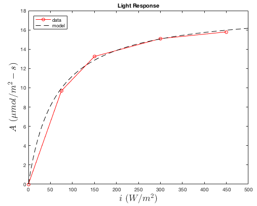
The response of photosynthesis to light is given by a simple exponential function, which is defined by only one parameter:

\(f_L(i) = \dfrac{i}{\theta+i}\),

where \(\theta\) is the light response curvature.

Temperature Response

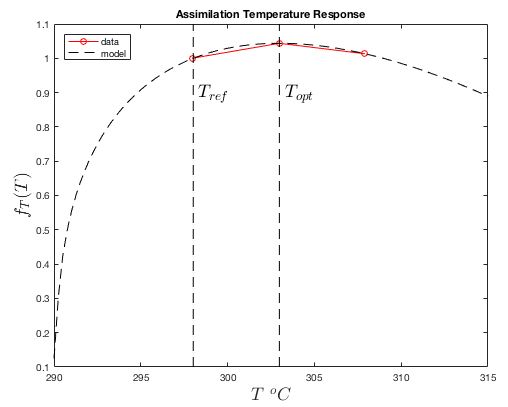
It is assumed that the maximum CO₂ assimilation rate \(A_{max}\) decreases exponentially about some optimum temperature \(T_{opt}\). The temperature response function is given by:

\(f_T(T_s) = \left(\dfrac{T_s-T_{min}}{T_{ref}-T_{min}}\right)^q\left(\dfrac{(1+q)T_{opt}-T_{min}-qT_s}{(1+q)T_{opt}-T_{min}-qT_{ref}}\right)\),

where \(T_{min}\) is the minimum temperature at which assimilation occurs, \(T_{opt}\) is the temperature at which the maximum assimilation rate occurs, \(T_{ref}\) is the reference temperature chosen to define \(A_{ref}\), and \(q\) is a shape parameter.

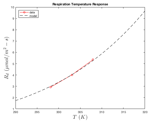
The "dark" respiration rate \(R_d\) is assumed to increase exponentially with temperature following the Arrhenius equation (and assumed not to vary with ambient CO₂ concentration). Thus, the dark respiration rate is calculated simply as

\(R_d = R\sqrt{T_s}\mathrm{exp}\left(-E_R/(T_s+273)\right)\),

where \(R\) and \(E_R\) are parameters, and temperature is in Kelvin.

CO2 Response Function

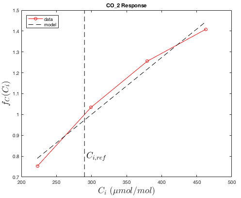
We assume that the maximum assimilation rate varies linearly with intercellular CO₂ concentration over the range of expected concentrations, and is zero at zero CO₂. Thus, the response function is simply

\(f_C(C_i) = k_C\dfrac{C_i}{C_{i,ref}}\),

where \(C_i\) is intercellular CO₂ concentration ( \(\mu\)mol CO₂/mol air).

Intercellular CO2 Concentration

The intercellular CO₂ concentration is estimated as a function of the boundary-layer conductance, stomatal conductance, and ambient CO₂ concentration outside of the primitive boundary-layer. The rate of transport of CO₂ to the leaf (i.e., assimilation rate) is given by

\(A = 0.75g_M\left(C_{amb}-C_i\right)\),

where \(g_M\) is the conductance to moisture from the sub-stomatal cells to outside of the boundary-layer. The 0.75 factor comes from the fact that diffusion of CO₂ in air is slower than that of water vapor (see Eq. 7.33 of Campbell and Norman).

Since \(A\) is dependent on \(C_i\) and vice-versa, an iterative solution is required for \(A\).

Empirical Model Calibration Procedure

Summary of Empirical Model Independent Variables

Variable	Units	Description
\(i\)	W/m²	Photosynthetic radiation energy flux.
\(T_s\)	Kelvin	Surface temperature.
\(C_{amb}\)	\(\mu\)mol CO₂/mol air	Ambient CO₂ concentration outside of boundary-layer.
\(g_{bl}\)	mol air/m²-s	Boundary-layer conductance.
\(g_s\)	mol air/m²-s	Stomatal conductance.

Summary of Empirical Model Parameters

Parameter	Units	Description
\(A_{sat}\)	mol CO₂/m²-sec	Assimilation rate at saturating irradiance and reference temperature and intercellular CO₂ concentration.
\(\theta\)	W/m²	Shape parameter for response to light.
\(T_{min}\)	Kelvin	Minimum temperature at which assimilation occurs.
\(T_{opt}\)	Kelvin	Temperature at which maximum assimilation rate occurs.
\(q\)	unitless	Temperature response shape function.
\(R\)	\({\mu}\)mol K^1/2/m²-s	Pre-exponential factor for respiration temperature response.
\(E_R\)	1/Kelvin	Respiration temperature response rate.
\(k_C\)	unitless	CO₂ response rate.

Response of Assimilation Rate to Light

The response of the assimilation rate to light is obtained from gas exchange measurements at reference temperature ( \(T_{ref}\)) and CO₂ ( \(C_{i,ref}\)) in which the irradiance is varied across some range. However, one important detail is that the dark respiration rate should be removed such that \(A=0\) in the dark (see plot below). This can be done by measuring the net CO₂ flux starting in the dark, then subtracting the dark flux from the total flux for each subsequent light level.

Light Response Curve

Response of Assimilation Rate to Temperature

The response of the assimilation rate to temperature is obtained using gas exchange measurements at saturating light levels and the reference CO₂ concentration. The temperature is varied across some range, and the assimilation rate is measured. It is assumed that the optimum temperature \(T_{opt}\) is the temperature corresponding to the maximum measured assimilation rate. The model is fit to the data to determine \(T_{min}\) and \(q\).

Temperature Response Curve

Response of Respiration Rate to Temperature

The response of the dark respiration to temperature is obtained using gas exchange measurements in the dark. The leaf is first acclimated to the dark chamber, then leaf temperature is varied across some range. The model is then fit to the data to determine parameters.

Respiration Response Curve

Response of Assimilation Rate to CO2

The response of the assimilation rate is obtained using gas exchange measurements at saturating light levels and the reference temperature \(T_{ref}\), but with varying external CO₂ concentration (which produces varying intercellular CO₂).

CO2 Response Curve

Dependencies	None
Python Import	`from pyhelios import PhotosynthesisModel`
Main Class	PhotosynthesisModel

Table of Contents