|
0.1.22
|
|
0.1.22
|
The following sections summarize past verification and validation efforts for Helios models. PyHelios provides Python bindings to these validated C++ implementations.
The Helios radiation model plug-in has automated verification tests that are run each time a new version of the code is committed to GitHub. These tests include both simple "toy problem" configurations with known analytical solutions, as well as more complex canopy architectures where theoretical solutions exist for certain metrics. The tests are implemented in plugins/radiation/tests/selfTest.cpp and are run using the doctest framework.
The radiation model has been verified against analytical solutions for several simple geometric configurations that do not involve complex canopy structures. These "toy problem" tests verify fundamental radiation transport physics including view factors, emission, reflection, and scattering.
90-Degree Common-Edge Squares: Two perpendicular square patches sharing a common edge are tested with both shortwave (collimated solar radiation) and longwave (thermal emission) bands. The test verifies proper handling of geometric view factors and reflection between surfaces at right angles.
Black Parallel Rectangles: Two parallel black rectangular patches separated by a known distance are used to test diffuse radiation exchange. The model results are compared against the analytical view factor solution for parallel rectangles, validating the Monte Carlo ray tracing accuracy for view factor calculations.
Gray Parallel Rectangles: An extension of the black rectangle test that includes non-unity emissivity and reflectivity values to verify proper handling of gray body radiation exchange and multiple scattering between surfaces.
Sphere Radiation Source: A spherical radiation source positioned above a rectangular patch tests the implementation of spherical radiation sources and verifies the geometric view factor calculation between a sphere and a planar surface using analytical solutions.
Second Law Equilibrium Test: An enclosed box with uniform temperature is used to verify that the radiation model satisfies the second law of thermodynamics. All surfaces in thermal equilibrium should emit exactly their black-body radiation times their emissivity, regardless of the complexity of multiple reflections within the enclosure.
Anisotropic Diffuse Radiation: Tests verify that horizontal patches receive the correct amount of diffuse radiation when anisotropic extinction coefficients are applied, ensuring proper implementation of directionally-dependent radiation attenuation.
All toy problem tests achieve Monte Carlo convergence with relative errors below 0.5% when averaged over 500 ensemble runs, demonstrating the accuracy of the fundamental radiation transport implementation.
For simplified canopy architectures, theoretical solutions exist for
1 - Canopy Light Interception: The homogeneous canopy patch test validates light interception calculations against Beer's law analytical solutions. A synthetic canopy is constructed with randomly positioned and oriented square leaf patches distributed throughout a 3D domain. The test compares both direct and diffuse radiation interception between model predictions and theoretical expectations.
For direct radiation at solar zenith angle \(\theta_s\), the theoretical canopy light interception follows:
\[I_{direct} = 1 - \exp\left(-\frac{0.5 \times LAI}{\cos(\theta_s)}\right)\]
For diffuse radiation, the theoretical interception integrates over all sky directions:
\[I_{diffuse} = \int_0^{\pi/2} 2\left(1 - \exp\left(-\frac{0.5 \times LAI}{\cos(\theta)}\right)\right) \cos(\theta) \sin(\theta) d\theta\]
The test creates a canopy with leaf area index (LAI) = 2.0, distributed over a 50m x 50m domain with 3m height. Ground-based radiation measurements and leaf-intercepted radiation are calculated within a central 40m x 40m area to minimize edge effects. Both direct (solar zenith angle = 36 degrees) and diffuse radiation scenarios are tested.
Model results demonstrate excellent agreement with theoretical predictions, with relative errors below 1% for both direct and diffuse radiation interception. This validates the accuracy of the Monte Carlo ray tracing implementation for randomly oriented surfaces in complex 3D canopy geometries (plugins/radiation/tests/selfTest.cpp:731).
2 - Canopy Sunlit/Shaded Leaf Area Fraction
Analytical expressions are available for calculating the fraction of sunlit and shaded leaf area, both in homogeneous canopies and in heterogeneous canopies. The equations for which are given in Bailey (2025).
The Beer's Law Tutorial in the native Helios documentation provides a detailed walkthrough of the sunlit-shaded leaf area calculation for a homogeneous canopy, which yields an agreement between Helios and the analytical solution with relative errors around 1%.
The figure below from Bailey (2025) shows the result for 3 different crown types. It should be noted that the theoretical solution has some error, particularly for the conical crown shape since it results in very short radiative path lengths that violate the assumptions of a turbid medium.
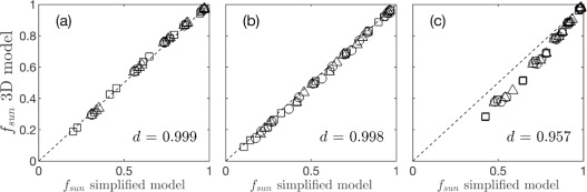
Figure. Comparison of theoretical model for \(f_{sun}\) and the value computed by the 3D model for four different single, isolated crown shapes: (a) spherical crown, (b) ellipsoidal crown, and (c) conical crown. Three different leaf angle distributions were simulated (spherical \(\circ\), planophile \(\triangle\), and erectophile \(\square\)). The dotted diagonal line corresponds to perfect 1:1 agreement.
3 - Canopy Absorbed Flux Probability Distributions
Analytical expressions for the probability distribution of absorbed direct, diffuse, and scattered radiation fluxes within a horizontally homogeneous canopy are given in Bailey and Fu (2022). This is a particularly strong verification test of the radiation model because it shows that it not only produces correct integrated fluxes, but also correctly predicts the probability distribution of fluxes across the canopy.
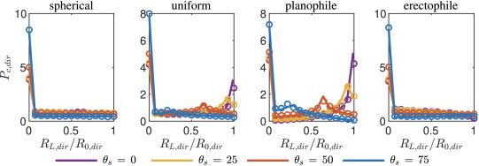
Figure. Probability density function of absorbed direct radiation flux within a horizontally homogeneous canopy of \(LAI = 1\). The absorbed direct radiation flux, \(R_{L,dir}\), is normalized by the incoming direct radiation flux on a surface perpendicular to the sun direction, \(R_{0,dir}\). Azimuthally isotropic leaf angle distributions of spherical, uniform, planophile, and erectophile are shown in each pane as indicated by the title. Each line corresponds to a different solar zenith angle. Open symbols correspond to the distribution obtained from 3D simulation.
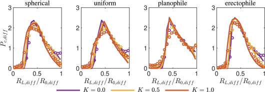
Figure. Probability density function of absorbed diffuse radiation flux within a horizontally homogeneous canopy of \(LAI = 1\). The absorbed diffuse radiation flux, \(R_{L,diff}\), is normalized by the incoming diffuse radiation flux on a surface perpendicular to the sun direction, \(R_{0,diff}\). Azimuthally isotropic leaf angle distributions of spherical, uniform, planophile, and erectophile are shown in each pane as indicated by the title. Each line corresponds to a different angular distribution of incoming diffuse radiation. Open symbols correspond to the distribution obtained from 3D simulation. In all cases shown, the solar zenith angle was 0 (vertical).
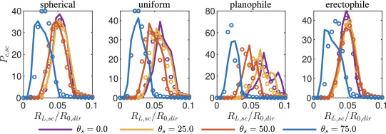
Figure. Probability density function of absorbed scattered radiation flux within a horizontally homogeneous canopy of \(LAI = 1\). Azimuthally isotropic leaf angle distributions of spherical, uniform, planophile, and erectophile are shown in each pane as indicated by the title. Each line corresponds to a different solar zenith angle. Open symbols correspond to the distribution obtained from 3D simulation. In all cases, the diffuse radiation fraction was \(f_{diff}\).
4 - ROMC Radiation Camera Tests
The radiation camera model has been verified against several tests from the ROMC benchmark suite. These tests involve comparing synthetic images generated by the radiation camera model against reference images for a variety of geometric and radiometric scenarios. Select results are given below, with more detailed description and analysis given in Lei et al. (2024).
| ROMC Test | SKILL Score |
|---|---|
| brfpp_uc_sgl | 98.00 |
| brfpp_co_sgl | 92.65 |
| brfop | 97.52 |
| fabs | 99.98 |
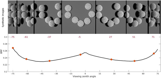
Figure. The bi-directional reflectance factor (BRF) curve of experiment HET51_DIS_UNI_NIR_00 measured in the ROMC case brfop and corresponding synthetic images captured by simulated cameras at multiple viewing zenith angles (red numbers below images).
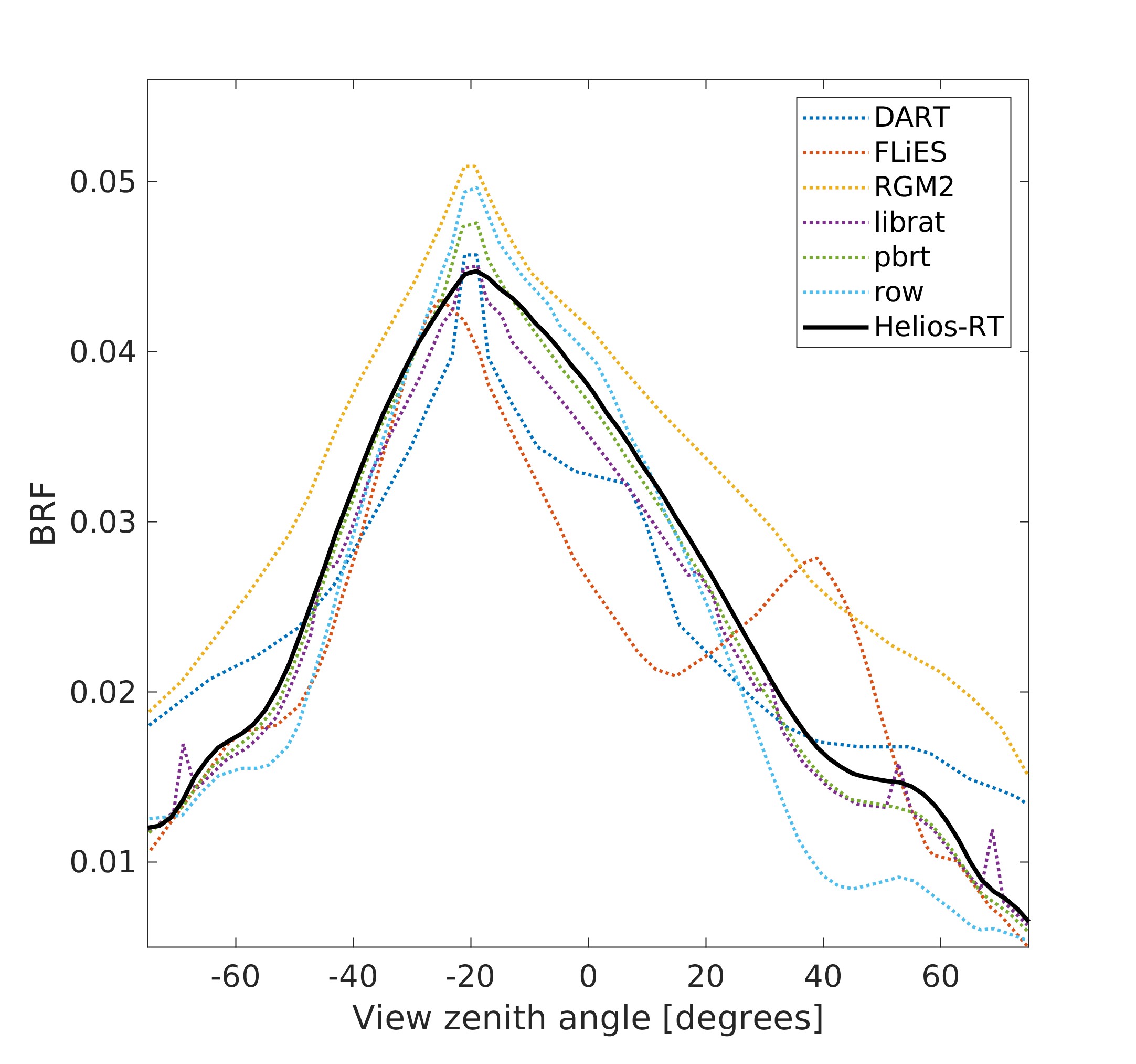
Figure. The BRF (brfpp) curves of the actual scene "Wellington Citrus Orchard" obtained by RAMI IV benchmark models and the present ray-tracing model (Helios-RT).
1 - Vineyard Canopy Light Interception
Ponce de Leon et al. (2025) conducted a field validation of the Helios radiation model in five different vineyard designs. Measurements consisted of differential measurements of all-wave solar radiation flux above and below the canopy. Results are summarized in the figure below.
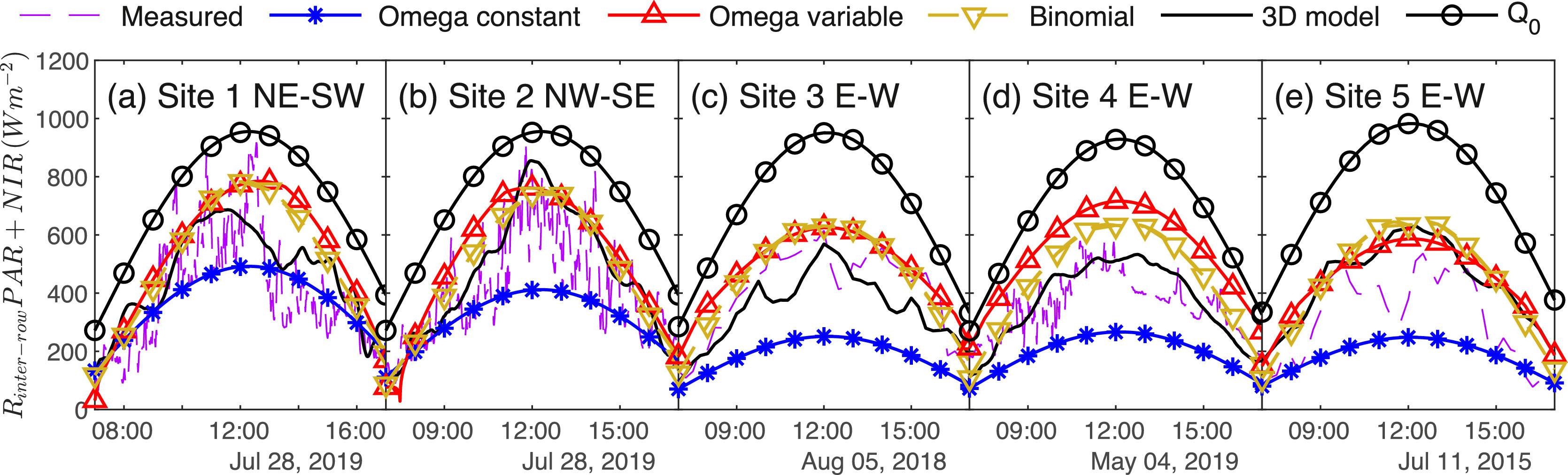
Figure. Measured and simulated radiation flux reaching the inter-row in the PAR and NIR band ( \(R_{inter-row}\)) in five different vineyard designs. This includes split grape canopy cases with rows orientated NE-SW (Site 1) and NW-SE (Site 2) at Barrelli Creek, Cloverdale CA; a double vertical grape canopy case with rows oriented E-W (Site 3) and a split canopy case with rows oriented E-W (Site 4) at Madera, CA; and a split grape canopy with rows oriented E-W in Lodi, CA (Site 5). Measurements and simulations were conducted every 1 min (Sites 1, 2, and 4) and every 15 min (Sites 3 and 5). The dashed magenta line is the measurement, and the solid black like is the Helios simulation. \(Q_0\) indicates the incoming radiation flux.
2 - Orchard Canopy Light Interception
Ponce de Leon et al. (under review) conducted a field validation of the Helios radiation model in an almond and olive orchard canopy. Measurements consisted of differential measurements of all-wave solar radiation flux above and below the canopy. Results are summarized in the figure below.
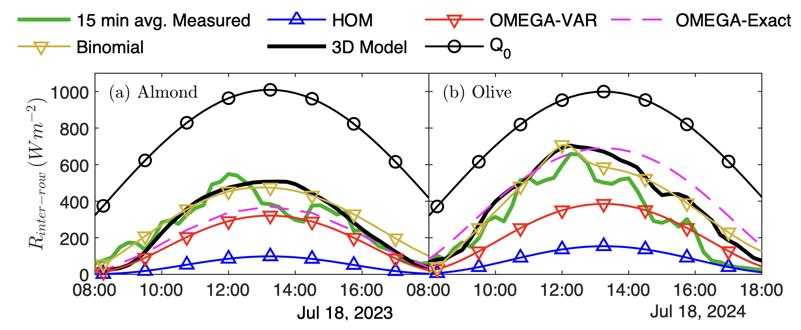
Figure. Measured and simulated 15-minute radiation flux reaching the inter-row in the PAR and NIR band ( \(R_{inter-row}\), W m-2) in an (a) almond orchard with rows orientated: NE-SW at Solano, CA on July 18, 2023 and in an (b) olive orchard with rows oriented N-S at Glenn, CA on July 18, 2024.
3 - Soybean Net Radiation Measurements
Wang et al. (2026) measured and validated net radiation based on measurements above a soybean canopy across a season. The model prediction agreed well with the measurements, with an overall R2 of 0.94.
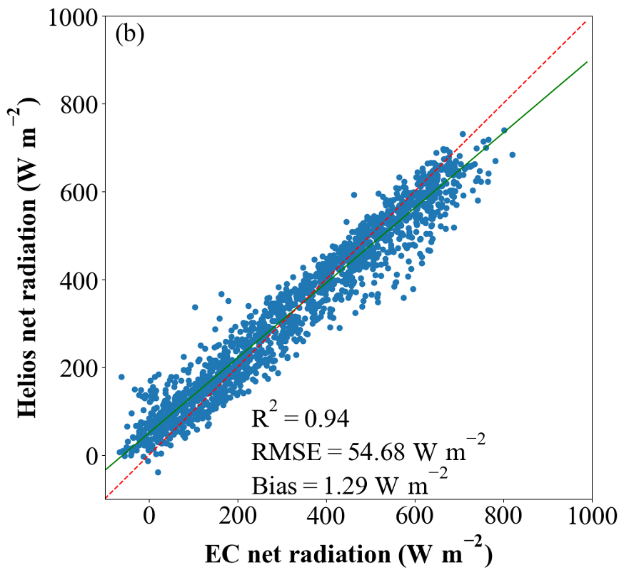
Figure. Validation of Helios net radiation against measurements of net radiation from an eddy covariance tower above a soybean canopy.
An important verification test of the energy balance model, aside from verifying energy balance closure, is to verify that the model satisfies the second law of thermodynamics. This is tested by setting the absorbed radiation flux of all elements in a simulated canopy scene to zero, and setting the longwave flux from the sky equal to \(\sigma T^4\), where \(T\) is an arbitrary temperature in Kelvin. After running the energy balance, all elements in the scene should have the same computed temperature of \(T\). This test is implemented in plugins/energybalance/tests/selfTest.cpp, and is explored in more detail in Bailey (2018).
1 - Grape Berry Temperature Measurements
Ponce de Leon and Bailey (2021)
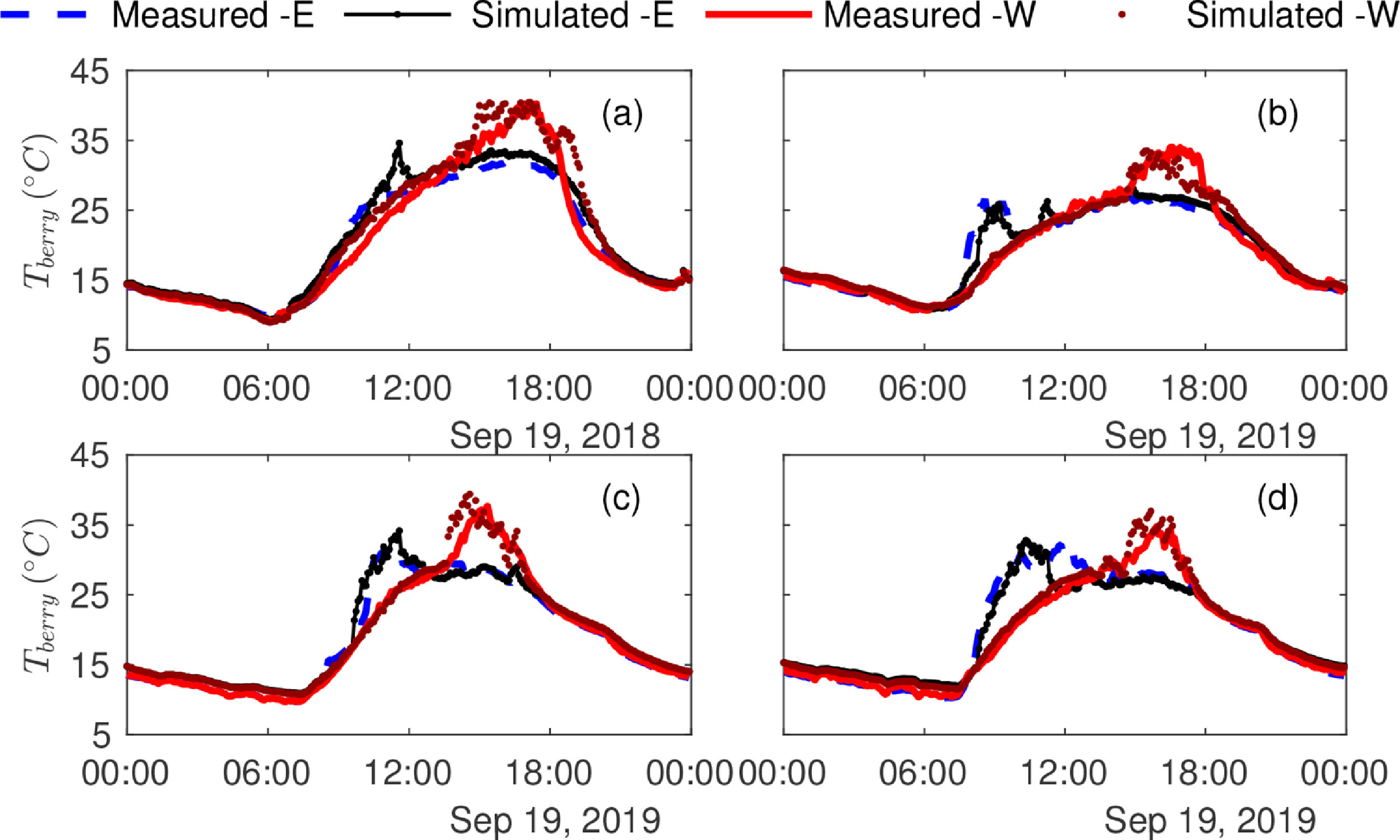
Figure. Daily course of simulated and average measured grape berry temperature in the east and west side of the vine for trellis systems (a) VSP, (b) Wye, (c) Goblet and (d) Unilateral.
2 - Cowpea Leaf Temperature Measurements
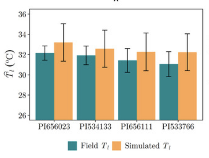
Figure. Measured and simulated cowpea leaf temperature (Tleaf, degrees C) for four different cowpea genotypes.
3 - Redbud Tree Leaf Temperature Measurements
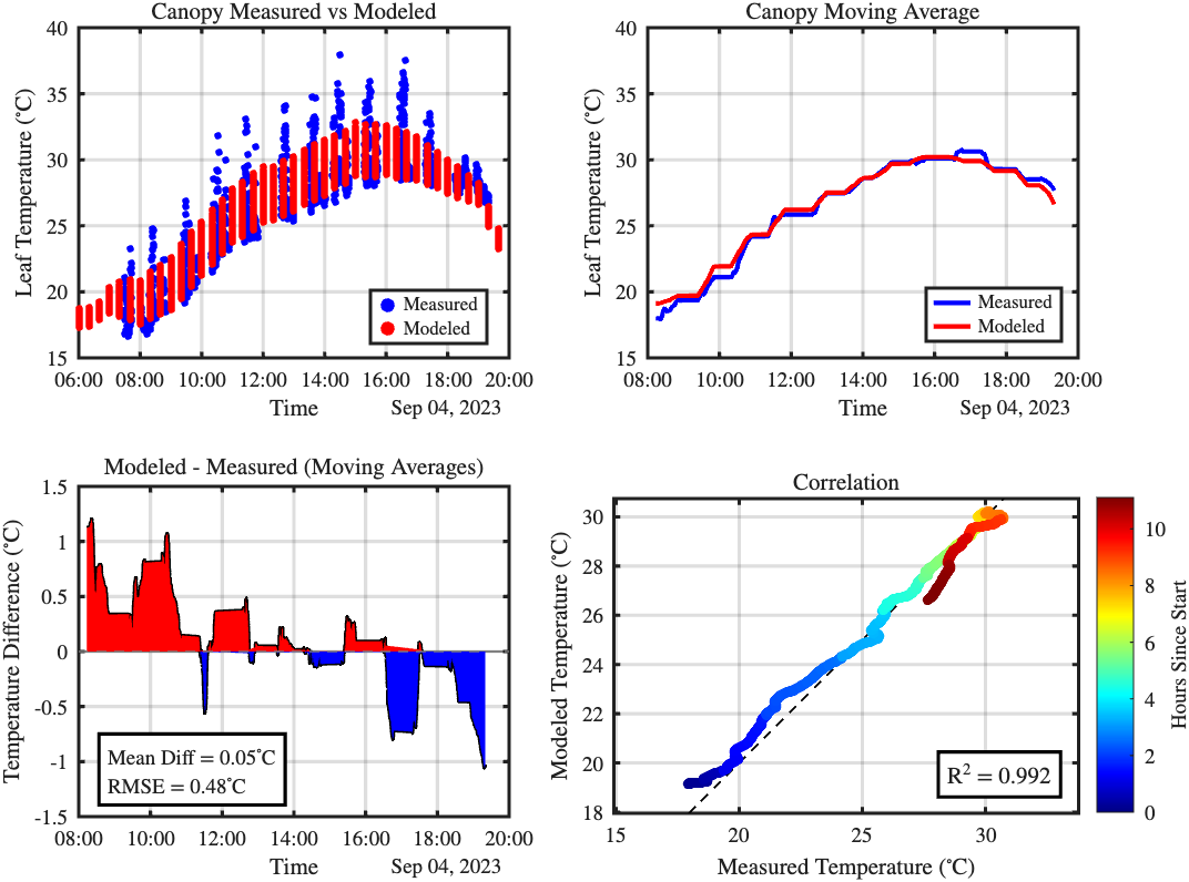
Figure. Comparison between simulated leaf temperature and an ensemble of measurements using a LICOR LI-600 porometer across a day.
1 - Almond Lysimeter Measurements
Whole-plant ET was validated in Helios by comparing against measurements of an almond tree in a weighing lysimeter. One Nonpareil almond tree was planted in a large weighing lysimeter at the Kearney Agricultural Research and Extension Center (KARE). The surrounding orchard consisted of 50% Nonpareil, 25% Wood Colony, and 25% Monterrey trees. Inputs for Helios included LiDAR scans for reconstruction, ambient weather data, and leaf-level gas exchange measurements.
The figure below shows validation results across two seasons, which indicate good model agreement. There are brief periods in which the experimental ET drops dramatically when irrigation is withheld during hull split, which was not explicitly represented in the simulations.
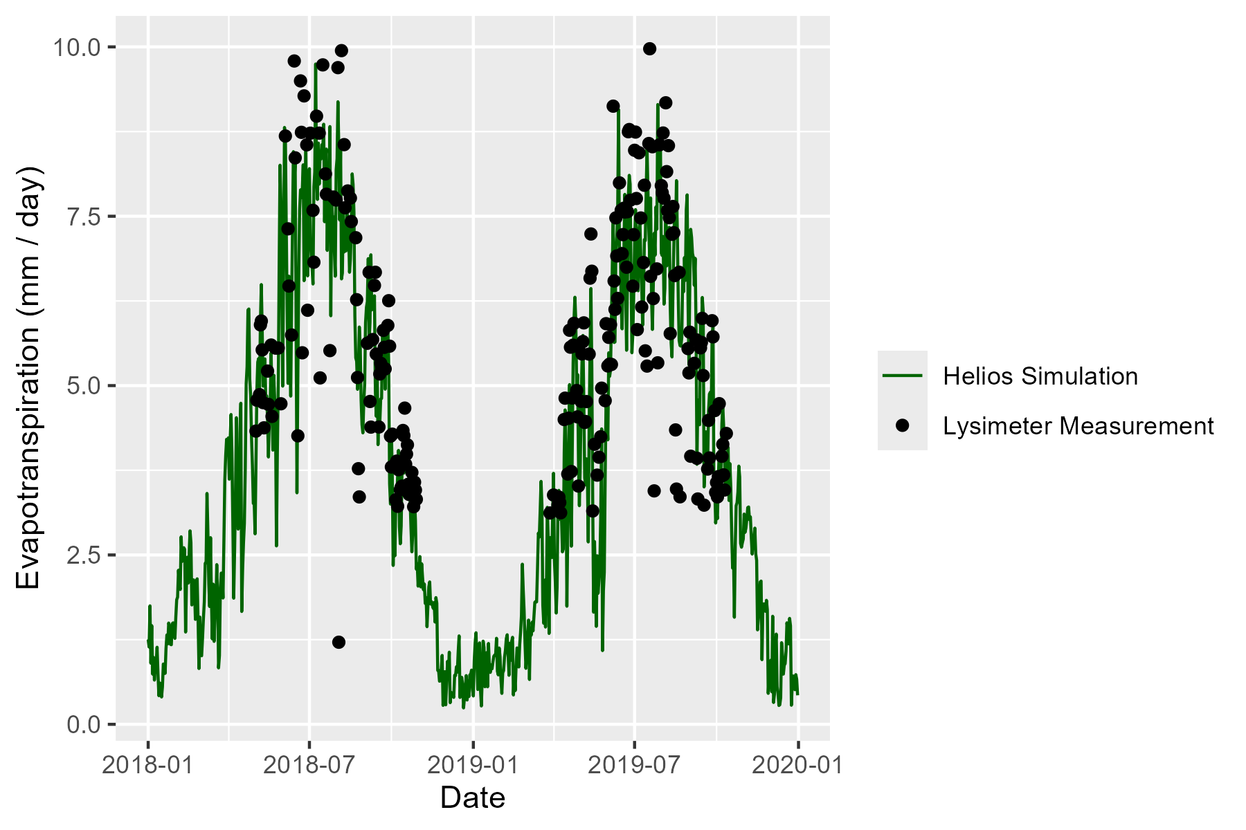
Figure. Validation of Helios whole-tree almond ET based on weighing lysimeter data.
1 - Soybean Eddy Covariance Measurements
Wang et al. (2026) validated Helios predictions of gross primary production (GPP) against measurements collected from an eddy covariance tower above a soybean field across a season.
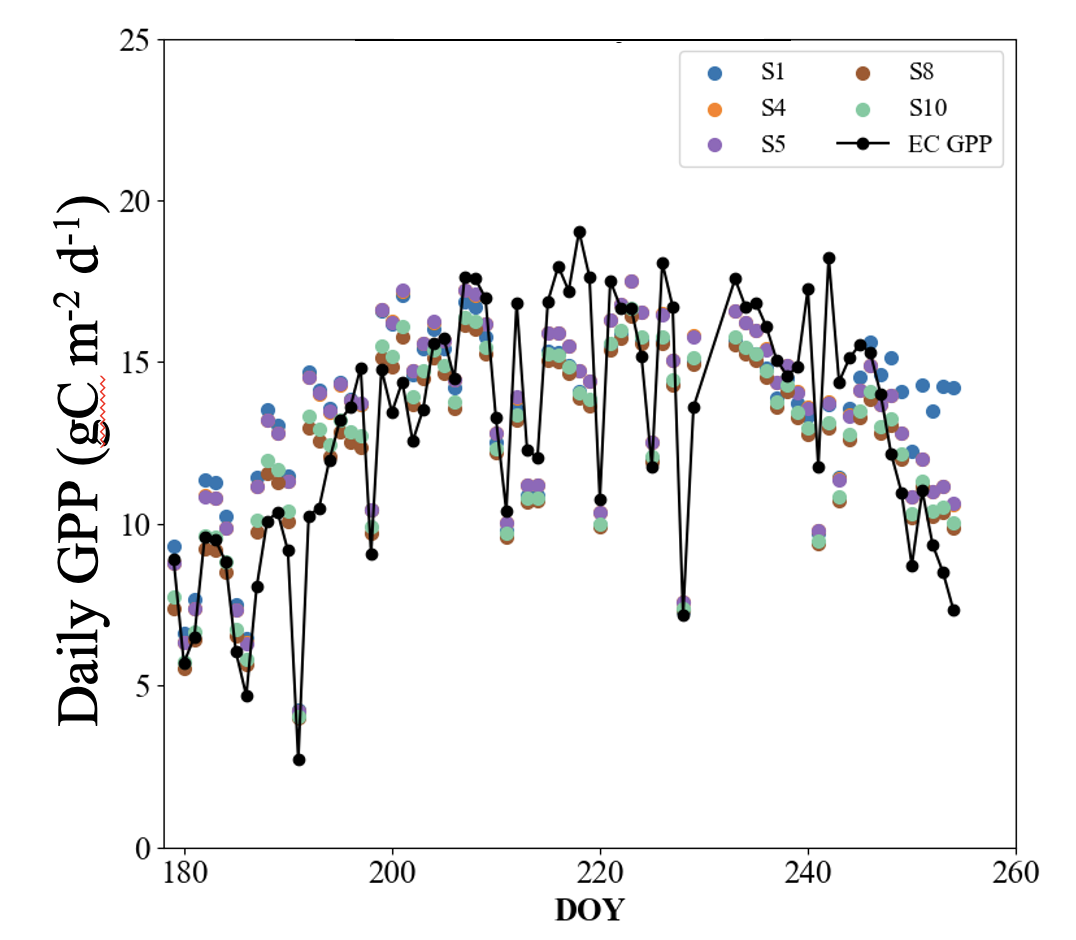
Figure. Validation of Helios against measurements of GPP collected from an eddy covariance tower above a soybean field across time. Different simulation lines correspond to a different scheme for representing spatial heterogeneity in photosynthesis parameters (see Wang et al. (2026) for details).
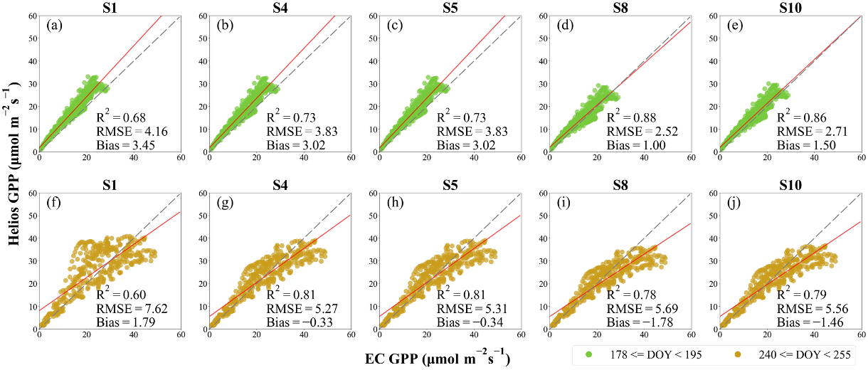
Figure. Validation of Helios against measurements of GPP collected from an eddy covariance tower above a soybean field. Each subplot corresponds to a different scheme for representing spatial heterogeneity in photosynthesis parameters (see Wang et al. (2026) for details). (a-e): performance for data from DOY 178 to DOY 195; (f-j): performance for data from DOY 240 to DOY 255.
The Helios LiDAR plug-in has many verification checks that are run each time a new version of Helios is released. These tests use synthetic LiDAR data to generate test data, where the exact scanned geometries are known, enabling accurate error calculations.
The leaf angle distribution calculations are verified by generating canopies of known leaf angle distribution, generating synthetic scan data based on them, then applying the leaf angle algorithm to the simulated data. A similar process is used to verify the leaf area inversion calculations.
Kent and Bailey (2024) conducted a detailed study of errors in Helios' LiDAR-based leaf area inversion using synthetic data, and estimated expected errors across a range of scenarios. Similarly, Halubok et al. (2022) used synthetic data to quantify errors in Helios' aerial LiDAR inversion of leaf area density.
1 - Leaf Angle Distribution Measurements
Bailey and Mahaffee (2017a) compared Helios-derived leaf angle distribution measurements from LiDAR data against manual measurements across a tree crown. Error in the LiDAR-based measurements was likely comparable to that of the manual measurements, as illustrated as part of the study. The paper highlights the importance of properly weighting LiDAR-derived leaf angles based on their projection in the direction of the scanner.
2 - Leaf Angle Distribution Method Intercomparison Study
Mutugi Murithi et al. (2025) performed an intercomparison study to evaluate different methods for estimating the leaf angle distribution from LiDAR data. The study concluded that the best performing algorithm was that used by Helios, which outperformed much newer algorithms both in terms of accuracy and in computational speed. The main failure of other methods is that they do not properly weight leaf angles based on their projection in the direction of the scanner, as recommended by Bailey and Mahaffee (2017a).
3 - Leaf Area Measurements
Bailey and Mahaffee (2017b) compared Helios-derived leaf area density measurements from LiDAR data against manually measured leaf area density in a tree. The index of agreement between LiDAR-derived and manually measured leaf area density was \(d=0.98\).