 |
1.3.77
|

| |
|
1.3.77
|
|
| |
| Dependencies | Visualizer plug-in CollisionDetection plug-in |
|---|---|
| CMakeLists.txt | set( PLUGINS "lidar" ) |
| Header File | include "LiDAR.h" |
| Class | LiDARcloud |
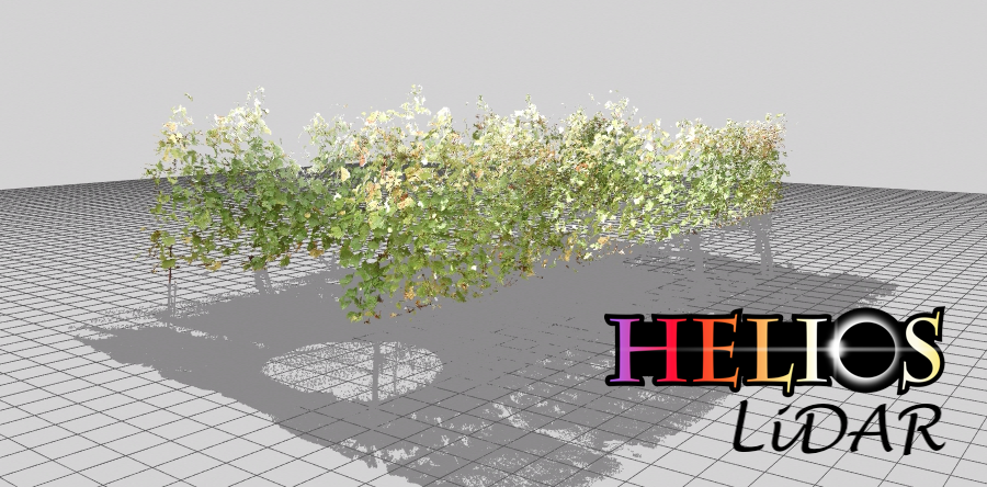
The LiDAR plugin is used to process terrestrial LiDAR data into information that is useful for plant models. For example, this may be to determine leaf area and angle distributions at the voxel scale, or to reconstruct individual leaves and add them to the Context.
The LiDAR plugin uses the CollisionDetection plugin for ray tracing. GPU acceleration is optional and controlled through the CollisionDetection plugin:
To enable GPU acceleration for faster processing of large point clouds:
isGPUAvailable() reports GPU capability, while isGPUAccelerationEnabled() reports whether acceleration is currently toggled on. Setting the HELIOS_NO_GPU environment variable forces the CPU path (isGPUAvailable() then returns false).
| Constructors |
|---|
| LiDARcloud( void ) |
The LiDARcloud class contains point cloud data, and is used to perform processing operations on the data. The class constructor does not take any arguments.
| Primitive Data Label | Symbol | Units | Data Type | Description | Available Plug-ins | Default Value |
|---|---|---|---|---|---|---|
| reflectivity_lidar | \(\rho_l\) | unitless | float | Primitive reflectivity in the waveband of the laser. This is used to calculate the return intensity in synthetic scans. | N/A | 1.0 |
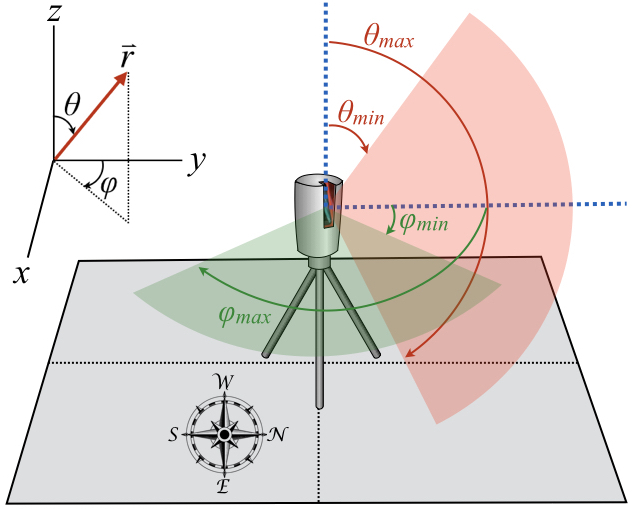
The algorithms associated with the LiDAR plug-in work with data obtained from a rectangular scan pattern. In this scan pattern, points are sampled at equally spaced intervals in both the zenithal ( \(\theta\)) and azimuthal ( \(\varphi\)) directions. At a given azimuthal angle, some range of zenithal angles are consecutively scanned, which represents a "scan line". Each scan line starts at some zenithal angle \(\theta\)min and ends at some zenithal angle \(\theta\)max. After recording a scan line at the first azimuthal angle \(\varphi\)min, the scanner incrementally moves to the next adjacent azimuthal scan direction and records the next scan line until it reaches the azimuthal angle \(\varphi\)max.
The number of zenithal points within each scan line is given by \(\mathrm{N}_{\theta}\), and the total number of scan lines (i.e., number of individual azimuthal directions) is given by \(\mathrm{N}_{\varphi}\).
Angles are typically specified as degrees. Distance units are arbitrary, but must be used consistently.
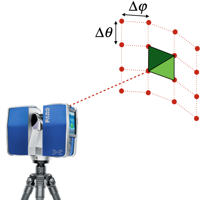
The laser beam emitted from a LiDAR instrument has some finite diameter, which increases with distance from the scanner. In many cases, the beam diameter may be larger than the width of individual leaves by the time it reaches the canopy. This means that a single laser pulse may intersect multiple objects along its path to the ground.
LiDAR data is commonly classified along two independent axes that are easy to conflate. The first is the instrument's detection method: a discrete-return instrument detects peaks in the returning signal in real time and records a small number of discrete points per pulse, whereas a full-waveform instrument digitizes and stores the entire returned signal as a function of time (the "waveform"), from which the individual returns are later extracted. The second axis is the number of returns recorded per pulse: single-return (one hit point per pulse) versus multi-return (several hit points per pulse, e.g. first, second, ..., last). These two axes are independent: discrete-return instruments routinely record multiple returns per pulse, and full-waveform instruments also ultimately output discrete returns once the waveform is decomposed.
The Helios LiDAR plug-in outputs discrete return points; it does not store or export a digitized waveform. Internally, however, synthetic multi-ray scans form an analytic waveform (a sparse sum of Gaussians, one per sub-ray hit) and detect returns from it, so the discrete points exhibit realistic signal-formation behavior such as range-resolution-limited merging and edge "ghost" points. What this documentation refers to throughout is the number of returns recorded per pulse:
Real instruments that produce multi-return data (such as the RIEGL VZ series) are often full-waveform internally, but the exported point cloud - and everything Helios simulates and processes - consists of discrete returns, not waveforms.
Synthetic scans select among three modes (see Generating Synthetic (Simulated) LiDAR Data): an idealized mode (one ray per pulse) that reports the exact ray-surface intersection; a limited (single/N)-return waveform mode; and an unlimited multi-return waveform mode. The number of rays per pulse selects idealized (1) versus waveform processing (more than 1), and the <returnMode> scan tag (or the syntheticScan() return-mode argument) selects limited versus unlimited return. In limited (<returnMode> single) mode the <maxReturns> tag sets the cap on returns per pulse: 1 = single-return (the default), 2 = dual-return, N = N-return; when a pulse resolves more returns than the cap, the <singleReturnSelection> policy chooses which to keep. A limited-mode pulse reports only real points (a transmitted-beam miss is recorded only when the pulse produces no real return), whereas unlimited multi-return mode records every detected return, including a transmitted-beam miss alongside real returns when miss recording is enabled - so multi-return mode is preferred when the resulting cloud will be used for leaf-area inversion.
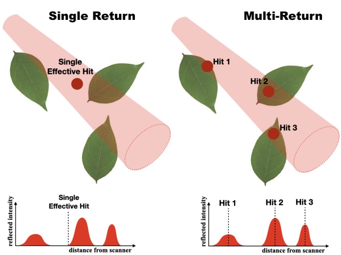
Each scan has a set of parameters or "metadata" that must be specified in order to process the data. Some parameters are optional, while some are required. The following metadata is needed to define the overall scan itself, in addition to individual scan hit points. Note that XML tags are case-sensitive.
The tags in the table below are common to all scan types. The tags that define the geometry of the scan depend on the scan pattern (selected with the <scanPattern> tag) and are listed separately for each pattern in Rectangular raster scan pattern and Spinning multibeam scan pattern below.
| Metadata | XML tag | Description | Default behavior |
|---|---|---|---|
| Scanner origin | <origin> | (x,y,z) coordinate of the scanner. This is the position where the scanner rays are sent from. Values should be separated by a space in the XML file. | None: REQUIRED |
| scan pattern | <scanPattern> | Geometric pattern of beam directions: raster (a uniform angular grid in zenith and azimuth - the default panoramic terrestrial-scanner pattern), spinning_multibeam (a rotating multi-channel sensor such as a Velodyne, Ouster, or Hesai unit), or risley (a rotating-Risley-prism rosette scanner, the optical mechanism of Livox rosette sensors such as the Mid-40/Mid-70/Avia). The geometry of each pattern is defined by additional tags listed in Rectangular raster scan pattern, Spinning multibeam scan pattern, and Risley-prism (Livox-style rosette) scan pattern below. | raster |
| translation | <translation> | Global (x,y,z) translation to be applied to entire scan, including the origin and all hit points. | No translation. |
| rotation (degrees) | <rotation> | Global spherical rotation (theta,phi) to be applied to the entire scan, including the origin and all hit points. | No rotation. |
| beam exit diameter (meters) | <exitDiameter> | Effective diameter of laser beam exiting the instrument. Only used for multi-return synthetic data generation. | 0 (single return) |
| beam divergence angle (rad) | <beamDivergence> | Angle of laser beam divergence after exiting the instrument. Only used for multi-return synthetic data generation. | 0 |
| range noise std. dev. (meters) | <rangeNoiseStdDev> | Standard deviation of zero-mean Gaussian noise added to the measured range (distance) of each return during synthetic scan generation. The hit point is displaced along the beam direction, producing realistic anisotropic positional error. Only used for synthetic data generation. | 0 (no noise) |
| angular noise std. dev. (rad) | <angleNoiseStdDev> | Standard deviation of zero-mean Gaussian jitter applied to the pointing direction of each pulse during synthetic scan generation. This produces the across-beam (lateral) component of the positional error, which grows with range. Only used for synthetic data generation. | 0 (no jitter) |
| scanner tilt (roll pitch, degrees) | <scanTilt> | Global scanner tilt applied to the entire scan frame about the scanner origin during synthetic scan generation. This models the residual tilt of the scanner spin axis away from true vertical (plumb) that a real terrestrial scanner's dual-axis inclinometer reports. Two angles are given, separated by a space: the first is the roll and the second is the pitch, applied in that order (roll first). The tilt uses a right-handed, Z-up body frame (matching commercial scanners such as those using the RIEGL SOCS convention): the body forward axis is the horizontal projection of the azimuth-zero ( \(\varphi\)min) scan direction, and the body lateral axis completes the right-handed frame. Roll is a right-hand rotation about the lateral axis; pitch is a right-hand rotation about the forward axis. When \(\varphi\)min=0 the lateral axis is world +x and the forward axis is world +y. Note that commercial scanners do not share a universal inclinometer sign convention, so when matching a specific instrument the sign should be verified against that instrument. Only used for synthetic data generation. | 0 0 (perfectly level) |
| scanner azimuth offset (degrees) | <scanAzimuthOffset> | Global scanner azimuth (heading) offset applied to the entire scan frame about the scanner origin during synthetic scan generation. This is the yaw component that completes the roll/pitch/yaw orientation of a real scanner: while <scanTilt> models the inclinometer roll and pitch, this models the compass heading of the instrument about the local vertical. It is a single angle giving a right-hand rotation about the world vertical (+z) axis, applied as a heading offset on top of the azimuth sweep [ \(\varphi\)min, \(\varphi\)max]. When combined with a tilt, the rotation order is yaw (azimuth) first, then pitch, then roll, so the azimuth offset also rotates the roll/pitch body frame. Note that commercial scanners do not share a universal heading sign convention, so when matching a specific instrument the sign should be verified against that instrument. Only used for synthetic data generation. | 0 (no offset) |
| return mode | <returnMode> | How a pulse reports detected returns during analytic-waveform synthetic scan generation (more than one ray per pulse): multi reports every detected return with no limit (discrete multi-return instrument), while single reports a limited number of points per pulse - at most <maxReturns> of them, selected by <singleReturnSelection>. In single-return mode (maxReturns 1) two surfaces within the pulse range-resolution blend into one return at an intermediate range, reproducing the "ghost"/"mixed pixel" point a real single-return instrument records at an edge. A single ray per pulse always produces an idealized exact intersection regardless of this setting. Note multi mode records a transmitted-beam miss alongside real returns (when miss recording is on), whereas single/N-return mode records a miss only for a fully transmitted pulse - prefer multi for leaf-area inversion. Only used for synthetic data generation. | multi |
| single-return selection | <singleReturnSelection> | Which return(s) are kept when <returnMode> is single and more returns than <maxReturns> are resolved: strongest (largest echo amplitude), first (nearest), or last (farthest). The kept returns are always reported nearest-first. Only used for synthetic data generation. | strongest |
| maximum returns per pulse | <maxReturns> | Maximum number of returns reported per pulse when <returnMode> is single: 1 = single-return, 2 = dual-return, N = N-return. When a pulse resolves more returns than this, the <singleReturnSelection> policy chooses which to keep (always ordered nearest-first). Must be at least 1. Ignored when <returnMode> is multi. Only used for synthetic data generation. | 1 (single-return) |
| pulse width / range resolution (meters) | <pulseWidth> | Range-resolution distance used to merge sub-ray hits into discrete returns during analytic-waveform synthetic scan generation: two surfaces closer than this distance fall within one transmit pulse and merge into a single return, reproducing the range-resolution (dead-zone) limit of a real instrument. Alternatively specify <pulseDuration> (seconds), which is converted via range = c·duration/2. When 0, the synthetic scanner uses the pulse_distance_threshold argument of syntheticScan() instead. Only used for synthetic data generation. | 0 (use syntheticScan argument) |
| detection threshold (energy fraction) | <detectionThreshold> | Minimum return energy fraction (range-normalized echo amplitude as a fraction of total per-pulse beam energy) for a return to be detected during analytic-waveform synthetic scan generation. Returns weaker than this are discarded, modeling the noise floor of a real instrument. Only used for synthetic data generation. | 0 (no suppression) |
| ASCII point cloud file | <filename> | File containing point cloud data to be read. | No file will be read. |
| ASCII file column format | <ASCII_format> | Labels for columns in ASCII point cloud file. See section below for possible values and examples. Labels should be separated by a space in the XML file. | x y z |
The default scan pattern (<scanPattern> raster </scanPattern>, or simply omitting the <scanPattern> tag) is a rectangular raster: a uniform angular grid of \(\mathrm{N}_\theta\times\mathrm{N}_\varphi\) beam directions spanning the zenith range [ \(\theta\)min, \(\theta\)max] and the azimuth range [ \(\varphi\)min, \(\varphi\)max]. This corresponds to a panoramic terrestrial laser scanner operating in gridded mode (e.g. RIEGL VZ, Leica, FARO Focus). The geometry is defined by the following tags, in addition to the common tags above:
| Metadata | XML tag | Description | Default behavior |
|---|---|---|---|
| size | <size> | Number of scan points in the theta (zenithal) and phi (azimuthal) directions, \(\mathrm{N}_\theta\) and \(\mathrm{N}_\varphi\). The two integers should be separated by a space. | None: REQUIRED |
| \(\theta\)min (degrees) | <thetaMin> | Minimum scan theta (zenithal) angle. \(\theta\)min=0 if the scan starts from upward vertical, \(\theta\)min=90 if the scan starts from horizontal, etc. | 0 |
| \(\theta\)max (degrees) | <thetaMax> | Maximum scan theta (zenithal) angle. \(\theta\)max=90 if the scan ends at horizontal, \(\theta\)max=180 if the scan ends at downward vertical, etc. | 180 |
| \(\varphi\)min (degrees) | <phiMin> | Minimum scan phi (azimuthal) angle. \(\varphi\)min=0 if the scan starts pointing in the +y direction, \(\varphi\)min=90 if the scan starts pointing in the +x direction, etc. | 0 |
| \(\varphi\)max (degrees) | <phiMax> | Maximum scan phi (azimuthal) angle. \(\varphi\)max=90 if the scan ends pointing in the +x direction, \(\varphi\)max=180 if the scan ends pointing in the -y direction, etc. NOTE: \(\varphi\)max can be greater than 360 if \(\varphi\)min > 0 and the scanner makes a full rotation in the azimuthal direction, in which case \(\varphi\)max = \(\varphi\)min + 360. | 360 |
Setting <scanPattern> spinning_multibeam </scanPattern> models a rotating multi-channel sensor (e.g. Velodyne, Ouster, Hesai), which is the most common pattern for mobile and UAV plant scanning. \(\mathrm{N}_\theta\) laser channels are each fixed at their own (generally non-uniformly spaced) elevation angle, and the whole head rotates continuously through 360 degrees while the platform moves along a trajectory. The pattern is represented internally as the same \(\mathrm{N}_\theta\times\mathrm{N}_\varphi\) scan table used by a raster scan, except that each row uses its channel's zenith angle (from <beamElevationAngles>) rather than a uniform step. Because the storage is shared, all downstream processing - ray tracing, hit tables, leaf-area and leaf-angle inversion - is identical to a raster scan. Each synthetic hit additionally records a channel data value giving the index of the laser channel (scan-table row) that produced it.
A spinning sensor is set up from its physical parameters - channel elevation angles, azimuth resolution, pulse repetition rate (PRF), and a platform trajectory - not from a hand-sized azimuth grid. The point count is determined by the PRF and the acquisition time, and the number of azimuth steps and revolution count are derived internally; you never specify an azimuth range, a number of azimuth steps, or a number of revolutions. See Moving-platform and spinning-multibeam scans (physical-parameter setup) below for the full setup, in both C++ (LiDARcloud::addScanSpinning()) and XML (the <azimuthStep>, <PRF>, and trajectory tags).
record_misses=true (see also Generating Synthetic (Simulated) LiDAR Data), which records the misses directly and does not rely on grid reconstruction.Setting <scanPattern> risley </scanPattern> models a rotating-Risley-prism scanner - the optical mechanism used by Livox rosette-pattern sensors such as the Mid-40, Mid-70, and Avia. A single beam is refracted through a stack of continuously rotating wedge prisms; when the prisms rotate at different (and generally incommensurate) rates, the exit beam traces a non-repetitive rosette that fills a circular field of view, denser toward the center. Each pulse's body-frame direction is computed by non-paraxial ray tracing - refracting the beam through both faces of each rotating wedge with the vector form of Snell's law - so the maximum deflection, and therefore the circular field of view, is an emergent property of the wedge angles and refractive indices rather than a directly specified parameter.
Because the pattern is non-separable (each pulse has its own direction as a function of time, not a row \(\times\) column angular grid), a Risley scan is stored as a single-row table ( \(\mathrm{N}_\theta = 1\)) with one column per pulse, and it is always trajectory-driven (like a spinning scan). The number of pulses is \(\mathrm{PRF}\times\) acquisition duration. Each synthetic hit records the moving-platform timestamp, pulse_id, and per-pulse origin_x/origin_y/origin_z (it does not record a channel, which is meaningful only for a spinning multibeam scan).
record_misses=true) so leaf-area inversion has the population of transmitted beams.A real mobile, UAV, or airborne instrument is set up from its physical parameters, not from a flattened angular grid. Helios provides first-class entry points that take those parameters directly and derive the internal sampling grid, rotation rate, revolution count, and per-pulse timing. A scan created this way is self-describing: query LiDARcloud::getScanMode(), LiDARcloud::getScanRotationRate(), LiDARcloud::getScanRevolutions(), and LiDARcloud::getScanStepsPerRev() to introspect it.
A spinning multibeam sensor rotates continuously through 360 degrees while the platform moves along a trajectory, so there is no partial-arc azimuth range - the only azimuth control is the angular resolution. Use LiDARcloud::addScanSpinning() with the physical instrument parameters:
Helios derives: rotation rate = PRF / (channels \(\times\) steps-per-rev); revolutions = rotation rate \(\times\) trajectory duration; the number of points = PRF \(\times\) duration; and the full multi-revolution azimuth sweep. Each pulse fires at the exact per-channel elevation.
A free-spinning sensor cannot be held at a fixed pose without overlapping itself, so there is no separate "stationary" entry point. For a stationary capture (a spinning sensor on a tripod), supply a trajectory of two coincident poses - the same position and orientation - separated in time by the acquisition duration. The time gap determines how long the sensor spins, and therefore how many revolutions it makes, exactly as for a moving capture.
For a non-spinning sensor carried on a moving platform, use LiDARcloud::addScanMovingRaster(): specify the per-frame angular fan resolution ( \(\mathrm{N}_\theta\times\mathrm{N}_\varphi\) over \([\theta_{min},\theta_{max}]\times[\varphi_{min},\varphi_{max}]\)), the trajectory, and the PRF, and Helios derives the per-pulse time sampling along the trajectory.
Use LiDARcloud::addScanRisley() with the physical optics of the prism head. Each prism is described by a RisleyPrism (wedge angle, glass refractive index, and rotor rate - the sign of the rotor rate sets the rotation direction, so a counter-rotating pair traces a rosette). The field of view is not specified directly; it emerges from the optics. Like a spinning scan, a Risley scan is always trajectory-driven, and a stationary capture is a trajectory of two coincident poses separated in time by the acquisition duration.
These scans can also be authored in a scan XML file. In addition to the common tags, a spinning multibeam scan uses:
| Metadata | XML tag | Description |
|---|---|---|
| azimuth resolution (degrees/step) | <azimuthStep> | Azimuth angular resolution in degrees per firing step. Required for a spinning scan; the number of azimuth steps per revolution and the total azimuth sweep are derived internally. |
| pulse repetition rate (Hz) | <PRF> | Laser firing rate. (Alias: <pulseRate>.) |
| lever arm (m) | <leverArm> | Sensor optical-center offset in the platform body frame, "x y z". |
| boresight (degrees) | <boresight> | Fixed sensor misalignment "roll pitch yaw". |
| trajectory (inline) | <trajectory> | Required for a spinning scan. A block of <pose> children, each "t x y z qx qy qz qw" (quaternion) or "t x y z roll pitch yaw" (Euler degrees). For a stationary "spin in place" capture, give two coincident poses (same position and orientation) separated in time by the acquisition duration. |
| trajectory (file) | <trajectoryFile> | Path to a whitespace-separated trajectory file (same row format as inline poses; '#' comment lines ignored), resolved relative to the XML file. |
A Risley-prism (risley) scan instead lists its rotating prisms. It uses <PRF>, the trajectory tags above, and:
| Metadata | XML tag | Description |
|---|---|---|
| rotating prism | <prism> | One per rotating wedge, in the order the beam passes through them: "wedgeAngle(deg) refractiveIndex rotorRate(Hz, signed) [phase(deg)]". The sign of the rotor rate sets the rotation direction; the optional fourth value is the initial clocking angle (default 0). At least one is required; a Livox-style sensor uses two counter-rotating prisms. |
| air refractive index | <refractiveIndexAir> | Refractive index of the medium surrounding the prisms (default 1.0). Optional. |
A stationary Livox-style rosette capture (two counter-rotating prisms), spinning in place for 0.5 s:
A moving (flight-line) spinning scan, with the trajectory in a referenced file:
A stationary spin in place: two coincident poses 2 seconds apart, so the sensor spins for 2 s at its derived rotation rate:
In addition to scan metadata, the data collected by the scan itself must also be added to the plug-in. This can be achieved by either reading data from an ASCII text file, or performing a synthetic scan. At a minimum, point cloud data consists of the Cartesian (x,y,z) coordinates of each hit in the scan. Additionally, hit points may also have an associated r-g-b color value, or some other scalar data value such as intensity or temperature.
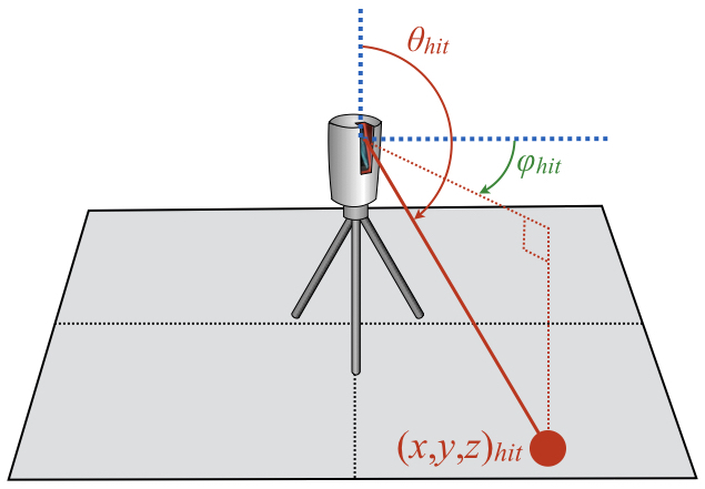
For the processing algorithms to work, the scan direction associated with each hit point must also be known. This can be specified directly as a ( \(\theta\), \(\varphi\)) spherical coordinate, or using the row (i.e., index in the scanline: 1... \(\mathrm{N}_\theta\)) and column (i.e., scanline index: 1... \(\mathrm{N}_\varphi\)). Otherwise, it will calculate the scan direction by drawing a line between the scan origin position and the hit point.
For multi-return data, additional information is needed about the hit points. Specifically, the total number of hit points along the pulse. The index can start at 0 or 1 for the first hit along the pulse, it just should be consistent for all points.
Scan metadata is typically specified by loading an XML file containing the relevant metadata for each scan. For real data, the XML file specifies the path to an ASCII text file that contains the data for each scan. For synthetic data, the parameters of the simulated scan are loaded from the XML file and used to perform the scan.
The code below gives a sample XML file for loading multiple scans. As specified in the metadata table above, not all entries are required (see above).
The ASCII text file containing the data is a plain text file, where each row corresponds to a hit point and each column is some data value associated with that hit point. The "ASCII_format" tag defines the column format of the ASCII text file (in this case, file.xyz). Each entry in the list specifies the meaning of each column. Possible fields are listed in the table below:
| Label | Description | Default behavior |
|---|---|---|
| x | x-component of the (x,y,z) Cartesian coordinate of the hit point. | None: REQUIRED |
| y | y-component of the (x,y,z) Cartesian coordinate of the hit point. | None: REQUIRED |
| z | z-component of the (x,y,z) Cartesian coordinate of the hit point. | None: REQUIRED |
| zenith (or zenith_rad) | Zenithal angle (degrees) of scan ray direction corresponding to the hit point. If "zenith_rad" is used, theta has units of radians rather than degrees. | Calculated from scan origin and hit (x,y,z). |
| azimuth (or azimuth_rad) | Azimuthal angle (degrees) of scan ray direction corresponding to the hit point. If "azimuth_rad" is used, phi has units of radians rather than degrees. | Calculated from scan origin and hit (x,y,z). |
| r (or r255) | red component of (r,g,b) hit color. If "r" tag is used, r is a floating point value between 0 and 1. If "r255" is used, r is an integer and between 0 and 255. | r=1 or r255=255 |
| g (or g255) | green component of (r,g,b) hit color. If "g" tag is used, g is a floating point value between 0 and 1. If "g255" is used, g is an integer between 0 and 255. | g=0 or g255=0 |
| b (or b255) | blue component of (r,g,b) hit color. If "b" tag is used, b is a floating point value between 0 and 1. If "b255" is used, b is an integer between 0 and 255. | b=0 or b255=0 |
| target_count | Number of hits along scan pulse. | Assumed to be single-return data. |
| target_index | Index of hit along scan pulse. | Assumed to be single-return data. |
| timestamp | Unique timestamp of hit point. | Assumed to be single-return data. |
| row | Scan-grid row index (zenithal/theta direction) of the hit point. Used by LiDARcloud::gapfillMisses() to reconstruct miss directions when timestamps are unavailable (see below). | N/A |
| column | Scan-grid column index (azimuthal/phi direction) of the hit point. Used by LiDARcloud::gapfillMisses() to reconstruct miss directions when timestamps are unavailable (see below). | N/A |
| deviation | Indication of variability in return within a given hit point. Note: this is never used for real data, but can be output for synthetic data. | N/A |
| echo_width | Range spread (width) of the return in meters: the transmit pulse range-extent combined in quadrature with the range spread of the surfaces that merged into the return. Note: this is computed for synthetic data only. | N/A |
| intensity | Range-normalized intensity of return, equal to \(\rho\,\cos\theta\) (per-primitive reflectivity times the incidence-angle cosine) with the \(1/R^2\) range loss of the LiDAR range equation normalized out, so it is independent of the scanner-to-target range. Note: this is never used for real data, but can be output for synthetic data. | N/A |
| reflectance | Synthetic return reflectance in decibels, \(10\,\log_{10}|I|\) where \(I\) is the range-normalized intensity, relative to a perfect Lambertian reflector at normal incidence (0 dB). Output only when "reflectance" is listed in the ASCII_format. Note: this is computed for synthetic data only. | N/A |
| (label) | User-defined floating-point data value. "label" can be any string describing data. For example, "temperature", etc. | N/A |
# x y z intensity reflectance. This makes the exported file self-describing and follows the conventional ASCII point-cloud header recognized by tools such as CloudCompare. The header is written by default; pass write_header = false to LiDARcloud::exportPointCloud() to suppress it. When loading, any line beginning with '#' is treated as a comment and skipped, so headered files round-trip without modification.The XML file can be automatically loaded into the point cloud using the LiDARcloud::loadXML() function, as illustrated below.
A hit point is flagged as a miss with the per-hit is_miss data value (1 = miss, 0 = return). You can satisfy the requirement in one of three ways, listed from most to least faithful to the original measurement:
| # | Approach | What you must provide in the imported ASCII file | When to use |
|---|---|---|---|
| 1 | Import the misses directly | An ASCII file that includes the no-return pulses, with an is_miss column (1 for the no-return pulses, 0 for returns) listed in the <ASCII_format>. Including row/column or timestamp as well is recommended but not required once is_miss is present. | Preferred. The true fired-beam geometry is used directly, with no reconstruction or assumptions. Requires that you can produce a file in which the no-return pulses survive (see below). |
| 2 | Reconstruct the misses with LiDARcloud::gapfillMisses() | A returns-only ASCII file that still carries either row and column scan-grid indices, or a per-return timestamp, in the <ASCII_format>. LiDARcloud::gapfillMisses() infers the empty (sky) directions of the scan grid from the returns and emits a miss for each (see Calculating leaf area for each grid cell for the two reconstruction strategies). | When you cannot export the no-return pulses but can export the row/column indices or timestamps. Works only for a regular raster scan grid. |
| 3 | Generate a synthetic scan with miss recording | Helios geometry plus a scan definition; call syntheticScan() with record_misses=true (see Generating Synthetic (Simulated) LiDAR Data). | When you are simulating, not importing, real data. Misses are recorded directly; this is the only option for non-raster (e.g. spinning-multibeam) patterns. |
If you import a returns-only file with none of is_miss, row/column, or timestamp, there is no information from which the miss directions can be recovered, and neither approach 1 nor 2 is possible. The triangulation, leaf-angle, and plant-reconstruction routines do not require misses and will still run, but the leaf-area inversion cannot. In that case you must re-export the data from the original instrument project so that the necessary information is retained, because it was discarded at export time and cannot be reconstructed afterward.
Helios imports plain ASCII/text point-cloud files (see LiDARcloud::loadXML() and the column table above); it does not read vendor binary formats (PTX, FLS, RDB, E57, LAS, etc.) directly. The task at export time is therefore to produce an ASCII file that satisfies approach 1 or 2 above. Exact menu names and options vary between software packages and versions, so the guidance below describes what capability to look for and how it maps to the Helios columns, rather than an exact click-path; verify the specifics against your software's current documentation.
XYZ with the "Include row/col" option enabled, which writes the scan-grid row and column index of each return as additional columns. This is an ordinary unstructured export - it contains only the returns, not the empty cells - but because every return is tagged with its grid row and column, LiDARcloud::gapfillMisses() can reconstruct the empty (miss) directions. Map those columns to the Helios row and column tokens in the <ASCII_format> (together with x, y, z and any intensity/color you want), then call LiDARcloud::gapfillMisses(). Including the intensity ("raw reflections") column as well is useful but not required. Exporting the structured PTX grid (see the Leica bullet below) is an alternative that additionally captures the empty cells explicitly, but it is not necessary when the row/column columns are available. 0 0 0 0) so that the full scan-line grid is preserved. (Ordered exports such as PTX retain the grid; unordered exports - XYZ Text, E57, PTS, etc. - do not, and drop the empty cells, unless they carry an explicit row/column column as in the FARO case above.) This is exactly the information Helios needs: the zero-coordinate cells are the misses, and a cell's position in the grid is its row and column. The practical workflow is to export the structured scan as PTX, then convert it to a Helios ASCII file with a short script that walks the PTX grid and writes, for each cell, the columns row column x y z plus is_miss (1 for a zero/no-return cell, 0 otherwise). With is_miss present you are using approach 1; with only row/column present you are using approach 2 and call LiDARcloud::gapfillMisses(). timestamp (mapped to the Helios timestamp column) along with x, y, z, and let LiDARcloud::gapfillMisses() reconstruct the miss directions. Because the exact attribute names and export options depend on the RiSCAN PRO / RiPROCESS version, confirm against the current RIEGL documentation that the timestamp (and, if available, a no-return flag you can map to is_miss) is included in the export. is_miss=1), or model the measurement as a synthetic scan in Helios with record_misses=true. is_miss flag or the row/column/timestamp columns, and check that those columns survive the round-trip and that the column order matches the <ASCII_format> tag used on import. (Helios writes a self-describing # header on its own ASCII exports; see the note above.) The example below shows the import-and-reconstruct workflow (approach 2) for a returns-only export that carries per-return timestamps:
If the file already contains the misses (approach 1, e.g. converted from a PTX grid), include is_miss in the <ASCII_format> and the LiDARcloud::gapfillMisses() call can be omitted:
Scans do not have to be defined in an XML file - they can also be created entirely in code through the API, which is useful when scan parameters are computed at runtime, when hit points come from another source, or when building automated tests. A scan is defined by constructing a Scan metadata object and registering it with LiDARcloud::addScan(), which returns the integer scan ID. Hit points are then added to that scan with addHitPoint().
The example below creates a rectangular raster scan, adds it to the point cloud, and adds a single hit point. The Scan metadata constructor takes the scanner origin, the grid resolution ( \(\mathrm{N}_\theta\), \(\mathrm{N}_\varphi\)), the zenith and azimuth ranges (in radians), the beam optics, the range and angular noise standard deviations, and the ASCII column format.
A spinning multibeam scan is created the same way, but with the Scan metadata constructor overload that takes a vector of per-channel zenith angles (in radians) in place of \(\mathrm{N}_\theta\) and the zenith range:
The addHitPoint() method has several overloads that additionally accept a hit color (helios::RGBcolor) and/or a map of named scalar data values (for example intensity, reflectance, or timestamp). For synthetic (simulated) scans, hit points are generated automatically by ray tracing the Helios geometry instead of being added by hand - see Generating Synthetic (Simulated) LiDAR Data.
Rectangular grid cells are used as the basis for processing point cloud data. For example, total leaf area (or leaf area density) may be calculated for each grid cell. Grid cells or "voxels" are parallelpiped volumes. The top and bottom faces are always horizontal, but the cells can be rotated in the azimuthal direction.
Grid cells are defined by specifying the (x,y,z) position of its center, and the size of the cell in the x, y, and z directions. Additional optional information can also be provided for grid cells, which are detailed below.
| Tag | Description | Default behavior |
|---|---|---|
| center | (x,y,z) Cartesian coordinates of cell center. | None: required. |
| size | Length of cell sides in x, y, and z directions. | None: required. |
| rotation | Azimuthal rotation of the cell in degrees. | 0 |
| Nx | Grid cell subdivisions in the x-direction. | 1 |
| Ny | Grid cell subdivisions in the y-direction. | 1 |
| Nz | Grid cell subdivisions in the z-direction. | 1 |
The grid cell subdivisions options allow the cells to be easily split up into a grid of smaller cells. For example, Nx=Ny=Nz=3 would create 27 grid cells similar to a "Rubik's cube".
Grid cell options can be specified in an XML file using the tags listed in the table above. Multiple grid cells are added by simply adding more <grid>...</grid> groups to the XML file.
Grid cells can also be added programmatically using the LiDARcloud::addGrid() function, without needing to specify them in an XML file. This is useful when grid parameters are computed at runtime or when setting up scans entirely in code.
The LiDARcloud::addGrid() function takes four arguments: the (x,y,z) center of the grid, the size of the grid in each dimension, the number of subdivisions in each dimension, and the azimuthal rotation angle in degrees.
This is equivalent to specifying the following in an XML file:
After adding the grid, you can query grid cell properties such as the cell size using LiDARcloud::getCellSize().
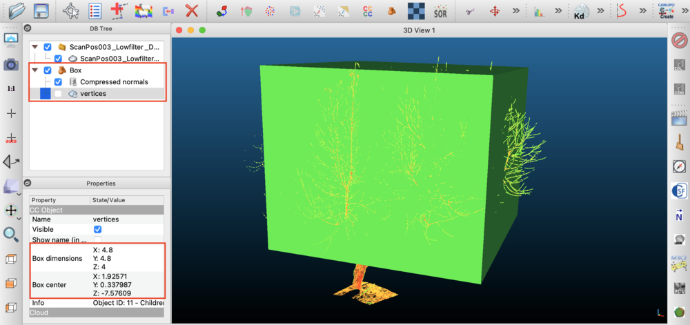
One way to figure out the appropriate dimension and position of the voxel grid is using the visualizer and trial-and-error. Make a guess of the voxel parameters, then visualize the point cloud and voxels together and adjust accordingly. This can be tedious and time-consuming because you need to re-run the entire code each time.
An often faster way to figure out the dimensions of the voxel grid is to use point cloud visualization software such as Cloud Compare. Load the point cloud data into Cloud Compare, then add a Box (file->Primitive Factory). You can translate or rotate the box by clicking on the Box object in the DB Tree pane, then select the menu item Edit->Translate/Rotate. To change the box size, click on the box vertices in the DB Tree pane, then go to Edit->Multiply/Scale. You can then find the resulting box location and dimensions in the Properties pane.
A triangulation between adjacent points is typically required for any of the available data processing algorithms. In the triangulation, adjacent hit points are connected to form a mesh of triangular solid surfaces. The algorithm for performing this triangulation is described in detail in Bailey and Mahaffee (2017a).
There are two possible options to be specified when performing the triangulation. A required option is \(L_{max}\), which is the maximum allowable length of a triangle side. This parameter prevents triangles from connecting adjacent leaves (i.e., we only want triangles to be formed with neighboring points on the same leaf). Typically we want \(L_{max}\) to be much larger than the spacing between adjacent hit points, and much smaller than the characteristic length of a leaf. For example, Bailey and Mahaffee (2017a) used 5cm for a cottonwood tree.
Another optional parameter is the maximum allowable aspect ratio of a triangle, which is the ratio of the length of the longest triangle side to the shortest triangle side. This has a similar effect as the \(L_{max}\) parameter, and works better in some cases.
The following code sample illustrates how to perform a triangulation.
Using the triangulation and defined grid cells, the plug-in can calculate the leaf area (and leaf area density) for each grid cell. The algorithm for calculating leaf area is described in detail in Bailey and Mahaffee (2017b) (except that in the current implementation, weighting by the sine of the scan zenith direction has been removed).
Performing the calculations is simple and requires no inputs, which is illustrated with the following code sample. Note that the leaf area calculation requires that the triangulation has been performed beforehand. If no triangulation is available, the plug-in will assume a uniformly distributed leaf angle orientation ( \(G=0.5\)). The leaf area calculation also requires that at least one grid cell was defined.
The leaf area calculation requires that the point cloud contains "miss" points: fired pulses that did not intersect any object and reached the sky. Misses count the laser beams transmitted through each voxel, which is the denominator of the transmission-probability inversion; without them the inversion is ill-posed, so LiDARcloud::calculateLeafArea() will raise an error if no misses are present. Many scanners do not record a hit point for a miss, so the misses must be supplied either by importing a scan format that retains them or by synthesizing them with the LiDARcloud::gapfillMisses() method (which infers the sky/miss directions from the recorded returns). Misses are flagged with the per-hit is_miss data field (1 = miss, 0 = return), which is set automatically by LiDARcloud::gapfillMisses() and syntheticScan(), and is carried through when present in imported data. If you are importing real scan data, see Miss points (transmitted beams) and how to export them for how to export your data from common instrument software (RIEGL, Leica, FARO, etc.) so that the misses - or the row/column/timestamp information needed to reconstruct them - are retained.
LiDARcloud::gapfillMisses() reconstructs the empty cells of the scan grid using one of two strategies, selected automatically per scan based on the data attached to the returns:
row and column hit data; preferred when both row/column and timestamp data are present). The native scan-grid indices give the 2D theta/phi raster directly. A robust per-row generative model is fit from the returns: each row's zenith is the median of the measured zeniths of its returns, and each row's azimuth is a robust (Theil-Sen) line fit \(\mathrm{azimuth} = \mathrm{intercept}[\mathrm{row}] + \mathrm{slope}[\mathrm{row}]\cdot\mathrm{column}\). The per-row azimuth offset/slope absorbs the continuous azimuth sweep (azimuth shear across rows) and the per-row zenith absorbs scanner tilt, without requiring the scan to be perfectly level or regular. Rows with too few returns (including entirely blank near-zenith rows) inherit their model parameters by robustly extrapolating the per-row parameters across the row axis, so large blank regions are extrapolated rather than only interpolated. This path does not require timestamps. The row/column indices are read from the ASCII columns of the same name (see the ASCII format table above). timestamp data but not row/column). The scan grid is reconstructed by sorting returns by timestamp and detecting sweep boundaries from the angular sequence, then interpolating/extrapolating along the inferred sweeps. If a scan's returns carry neither row/column nor timestamp data, LiDARcloud::gapfillMisses() raises an error, since there is no information from which to reconstruct the miss directions. (A scan containing no returns at all is skipped gracefully.)
In addition to the leaf-area point estimate, the plug-in can quantify the statistical sampling uncertainty of the per-voxel leaf area density (LAD), following Pimont et al. (2018). Each voxel is sampled by a finite number \(N\) of beams, so the transmittance statistic used in the inversion has sampling variance that depends on \(N\), the optical depth, the spread of beam path lengths, and the size of the vegetation elements. The variance has two components: a finite-beam sampling term that decays as \(1/N\), and an \(N\)-independent term arising from the variability of element positions within the voxel.
The element-position variance term requires a characteristic vegetation element width (e.g. mean leaf width), supplied as an optional argument to calculateLeafArea(). If a non-positive width is passed, that term is omitted and the reported uncertainty is sampling-only. The leaf-area point estimate is identical regardless of this argument.
Single-voxel confidence intervals are routinely \(\pm 50\)- \(100\%\) and are only valid in specific \((L, L_1, N)\) ranges (Pimont et al. 2018, Table 3); the accessors refuse to emit an interval outside that envelope. The recommended path is the group-scale interval (LiDARcloud::getGroupLADConfidenceInterval), which aggregates over a set of voxels (a vertical slice, a whole plant) and yields much tighter intervals ( \(\pm 5\)- \(10\%\)).
The per-voxel sufficient statistics are also available individually via LiDARcloud::getCellBeamCount, LiDARcloud::getCellRelativeDensityIndex, LiDARcloud::getCellMeanPathLength, and LiDARcloud::getCellLADVariance (which is the sampling variance of LAD in \((1/m)^2\), or \(-1\) where undefined).
A leaf-by-leaf reconstruction can be performed for the plant of interest using the method described in Bailey and Ochoa (2018). The reconstruction utilizes the triangulation and leaf area computations to ensure the correct leaf angle and area distributions on average, and thus requires that these routines have been run before performing the reconstruction.
There are two types of available reconstructions. One is a triangular reconstruction that directly uses triangles resulting from the triangulation to produce the reconstruction. The advantage is that it does not require any assumption about the shape of the leaf and can give a more direct reconstruction in some cases, however this reconstruction is typically not recommended as it often results in many small triangle groups that don't necessarily resemble actual leaves. This reconstruction is performed using the LiDARcloud::addReconstructedTriangleGroupsToContext(helios::Context*) const function, whose arguments are thresholds for the minimum and maximum area of reconstructed triangular leaf groups.
The other type of reconstruction is the "Alpha Mask" reconstruction, which replaces the triangle groups with a "prototype" leaf (which is an alpha mask). This ensures that all reconstructed leaves are representative of an actual leaf in terms of shape and size. This reconstruction is performed using the LiDARcloud::leafReconstructionAlphaMask( float, float, float, const char*) function. This function's arguments, in addition to area thresholds, are the aspect ratio of the prototype leaf (length along midrib divided by width perpendicular to midrib) and the path to a PNG image file to be used for the leaf alpha mask.
There is a function that can automatically add all reconstructed elements (triangles or alpha masks) to the Helios Context, which is LiDARcloud::addLeafReconstructionToContext().
Below is an example of performing a reconstruction using alpha masks and adding the alpha masks to the Context.
The LiDAR plug-in can simulate single-return and multi-return measurements based on the geometry in the Context. Ray-tracing is used to simulate the emission of radiation from the instrument, and based on ray-object intersection tests with primitive geometry in the model domain, the simulated hit points can be determined. Both the rectangular raster and spinning multibeam scan patterns are supported (see Rectangular raster scan pattern and Spinning multibeam scan pattern). Note that the simulated output consists of discrete return points; Helios does not generate or store a digitized waveform (see Single-return vs. multi-return LiDAR data).
To simulate single-return data, each laser pulse is modeled by a single ray emanating from the scanner origin. Rays are launched according to the scan parameters currently specified in the LiDARcloud. After calling the appropriate synthetic scan generation function (see below), the simulated scan data will be added to the LiDARcloud as if it was imported from real LiDAR data. In addition to the (x,y,z) location of the ray intersection, the model also produces estimates of return intensity, deviation, and can return an identifier for the intersected object.
reflectivity_lidar, default 1) and \(\theta\) is the angle between the laser beam and the surface normal at the hit point. This is the angular (incidence-angle) and reflectivity content of the LiDAR range equation. The intensity reported by Helios is range-normalized: the \(1/R^2\) geometric loss that a real instrument's return amplitude incurs over the scanner-to-target range \(R\) is normalized out, so a given surface produces the same intensity regardless of how far it is from the scanner. Equivalently, Helios reports the range-independent backscatter amplitude rather than the raw range-dependent signal a physical detector would record. For multi-return scans, the partial-footprint attenuation of sub-footprint targets is retained implicitly through the fraction of beam sub-rays that strike the target, as this reflects a target property rather than a range-geometry loss. The model does not currently include atmospheric attenuation, transmitted-pulse energy, detector gain, leaf transmittance, or multiple scattering.If the ASCII_format of the scan includes the reflectance tag, the scanner additionally records the return reflectance in decibels, \(10\,\log_{10}|I|\), where \(I\) is the range-normalized intensity described above. This follows the convention used by terrestrial laser scanners (e.g. RIEGL), in which reflectance is reported relative to a perfect Lambertian reflector viewed at normal incidence: such a target has \(I = 1\) and therefore a reflectance of 0 dB, while all real returns are negative. Returns with no detectable signal (misses, fully grazing, or back-facing hits) are floored at a large negative value rather than \(-\infty\), mirroring a scanner's minimum detectable reflectance. The reflectance tag is meaningful only for synthetic scans; for imported real data the reflectance values come from the data file as-is.
For multi-return data simulation, multiple sub-rays are cast for a single laser beam pulse, spread over the beam divergence cone and (if a finite <exitDiameter> is given) the exit aperture. Each sub-ray carries a Gaussian footprint weight \(w=\exp(-2(r/r_0)^2)\) set by its offset \(r\) from the beam axis (with \(r_0\) the 1/e \(^2\) radius), so the beam has the Gaussian transverse irradiance profile of a real laser rather than a uniform "top-hat". These weights drive the energy-weighted range and intensity of each detected return.
The sorted sub-ray hits are treated as an analytic sum-of-Gaussians waveform (each hit is a Gaussian of range-extent equal to the pulse range-resolution and amplitude \(w\cos\theta\)), from which discrete returns are detected:
pulse_distance_threshold argument when <pulseWidth> is 0) are unresolved and merge into a single return at the energy-weighted range. Two surfaces within one pulse width therefore blend into one return at an intermediate range - the physical origin of an edge "ghost"/"mixed pixel" point.single) exactly one return per pulse is reported, chosen by <singleReturnSelection> (strongest, first, or last); in multi-return mode (the default) every surviving return is reported.Note that single-return waveform mode is no cheaper than multi-return: the full sub-ray bundle is still traced to form the waveform; only the idealized one-ray-per-pulse mode avoids the bundle. In addition to the target count, target index, and timestamp, each hit point records an echo_width (the pulse-range-extent combined in quadrature with the range spread of the merged surfaces).
To generate synthetic single-return LiDAR data, first add all desired model geometry to the Context. Then declare an instance of the LiDARcloud class as above, and load an XML file containing the scan parameters. As in the case of importing a real point cloud dataset, the XML file must specify the scan origin and the scan resolution at a minimum (see above). However, in the case of synthetic data generation, you will not specify a filename to read containing point cloud data, as this data will be generated by the simulation. You can optionally specify the ASCII_format tag, which will determine which additional data fields should be recorded for each hit point. Valid hit point data fields are listed above in Loading scan data from file. If you specify the name of a user-defined scalar data field as a column in the ASCII_format tag, the synthetic scan will label each hit point with the value of that data field for the intersected primitive. The label is resolved from the intersected primitive's primitive data first; if the primitive has no primitive data of that name, the scanner falls back to the object data of the primitive's parent compound object. This lets a hit be labeled with a field carried either per-primitive or by the parent object (for example, a per-object classification or branch order). When a label exists on both, the more specific per-primitive value is used. For example, if the field "temperature" is listed in the ASCII_format tag, the value of primitive data (or, failing that, object data) "temperature" for the primitive corresponding to each hit point is recorded. Only scalar data types (float, double, int, uint) can be transferred to a hit point; non-scalar types (vectors, strings) and labels that exist on neither the primitive nor its parent object are skipped for that hit.
If no ASCII_format tag is provided in the XML file, the default is to record the (x,y,z) position of the hit point. If the function LiDARcloud::exportPointCloud() is called, it will export the simulated point cloud according to the provided ASCII_format tag (or the default if not provided).
Note that you can add multiple <scan></scan> blocks in a single XML file to perform multiple scans.
Once the LiDARcloud has been declared, and an XML file containing the scan parameters has been read, a single-return synthetic scan can be performed by calling LiDARcloud::syntheticScan(helios::Context*). This version (i.e., without the optional rays_per_pulse and pulse_distance_threshold arguments) will perform a single-return synthetic scan.
The code block below gives an example XML file. As a reminder, you can place this XML file anywhere, but the path given to the LiDARcloud::loadXML() function should either be absolute or relative to the directory in which the executable is being run (usually build/).
Example code is given below for generating synthetic single-return data and writing to an ASCII text file.
Generation of synthetic multi-return data is similar to single-return, except that additional information is needed to define the scan and simulation. In the XML file, the user must specify the diameter of the laser beam at the scan origin using the <exitDiameter> </exitDiameter> tags, as well as the angle of beam divergence in radians using the <beamDivergence> </beamDivergence> tags. If the exit diameter value is not specified, the default value of 0 is used, which means that the model will revert to single-return data generation. If the beam divergence value is not specified, a default beam divergence of 0 will be assumed, which effectively just means that the beam will remain perfectly cylindrical with diameter of exitDiameter.
Contents of an example XML file is given below.
Running the synthetic data generation function requires the specification of parameters associated with the simulation. The first is the number of rays to use per laser pulse in performing ray-tracing calculations, which sets the maximum possible number of hits possible per pulse. Specifying 1 ray/pulse effectively creates a single-return simulation, because that would mean you could only have a maximum of 1 hit/pulse. Ideally, you want a large number of rays/pulse because it allows for more hits/pulse if needed and results in more accurate simulations. The drawback to a very high number of rays/pulse is that the simulation will take longer to run. A value on the order of 100 is usually reasonable.
Second, the user needs to specify the distance threshold for aggregation of similar ray hit distances. For each simulated laser pulse, the number of rays/pulse specified above are launched from the scan origin. When some or all of those rays intersect the same surface, they will record a distance from the scanner to the hit point that is slightly different for each ray. Similar distances, which are presumed to lie on the same surface, are aggregated into a single hit point if they are within this distance threshold of each other. This is similar to how a real LiDAR instrument works as indicated in the sketch above, in that it aggregates similar returns into a single hit point. Specifying too small of a distance threshold may result in many duplicate hit points on the same surface. Specifying too large of a threshold may result in hit points that lie in between two disconnected surfaces (e.g., leaves). A threshold value that is smaller than the leaf or branch with is usually reasonable.
Below is example code with a rays/pulse value of 100 and distance threshold of 0.02.
Synthetic hit points can be labeled based on the primitive they intersect based on the value of the primitive data "object_label" of type 'int'. Primitive groups can be labeled in any way by setting a common integer value for the "object_label" primitive data. In order to enable synthetic data labeling, the column "object_label" must be included within the <ASCII_format> tag in the scan XML file. The object_label value for each hit point will be recorded and a column will be written if the point cloud is exported to file.
Miss recording is enabled by calling the overload that exposes the record_misses argument and passing true. There is no need to call LiDARcloud::gapfillMisses() afterward: the misses are recorded directly along their true fired-beam directions, each flagged with is_miss=1, so no grid reconstruction is involved (this is also the only way to obtain misses for non-raster patterns such as spinning multibeam, where LiDARcloud::gapfillMisses() does not apply). The companion scan_grid_only argument is an independent memory optimization (it restricts recording to rays that intersect the voxel grid) and can be left false.
record_misses off. It is specifically the leaf-area (gap-fraction) inversion that needs them.By default, synthetic hit points lie exactly on the surface that the ray intersects. Real LiDAR instruments have finite measurement precision, so each recorded point contains random error. This error is anisotropic — it does not scatter equally in all three Cartesian directions — and is naturally decomposed into two components that act along orthogonal axes of the per-point error ellipsoid:
Adding isotropic noise directly to the (x,y,z) coordinates would not be physically realistic. The two components are configured independently:
Range noise. Specify the standard deviation of the range error (in meters) using the <rangeNoiseStdDev> </rangeNoiseStdDev> tags. During synthetic scan generation, the measured range of each return is perturbed by an independent zero-mean Gaussian draw with this standard deviation, and the hit point is reconstructed along the nominal beam direction. The recorded "distance" data value reflects the noisy range. Typical terrestrial laser scanner range precision is on the order of 0.002–0.012 m.
Angular jitter. Specify the standard deviation of the pointing error (in radians) using the <angleNoiseStdDev> </angleNoiseStdDev> tags. During synthetic scan generation, the nominal direction of each pulse is perturbed by an independent zero-mean Gaussian angular offset with this standard deviation before ray tracing, so the whole beam — including any divergence cone and finite aperture — is rotated together. Because the displacement scales with range, this is the across-beam component of the error ellipsoid.
Misses are not perturbed by either term. If a tag is omitted (or set to 0), that component is disabled; with both omitted, points lie exactly on the surface (the previous behavior). The appropriate magnitudes should be taken from the instrument datasheet.
For example, to emulate an instrument with a 3 mm range precision and 0.2 mrad pointing jitter:
Results can be visualized using the Visualizer plug-in for Helios. There are two possible means for doing so. First, is to add the relevant geometry to the Context, then visualize primitives in the Context using the Visualizer. This works for the triangulation and plant reconstructions, but cannot be used to visualize just the point cloud since there is no "point" primitive in the Context. The next section describes how to accomplish this.
The second option is to add any geometry directly to the Visualizer. There are several functions build in to the LiDAR plug-in that can to this automatically, which are listed below.
| Function | Description |
|---|---|
| LiDARcloud::addHitsToVisualizer | Add all hits in the point cloud to the visualizer. |
| LiDARcloud::addGridToVisualizer(Visualizer*) const | Add all grid cells to the visualizer, which are displayed as translucent voxels. |
| LiDARcloud::addTrianglesToVisualizer | Add all triangles to the visualizer, which are colored by the r-g-b color value. |
| LiDARcloud::addTrianglesToVisualizer | Add triangles from a specified grid cell to the visualizer, which are colored by the r-g-b color value. |
The following code sample illustrates how to visualize the point cloud.
Results of data processing can be easily written to file for external analysis. The following table lists these functions. Data is written to an ASCII text file, where each line in the file corresponds to a different data point (e.g., hit point, triangle, etc.).
| Function | Description |
|---|---|
| LiDARcloud::exportPointCloud( const char* filename, bool write_header ) | Write the entire point cloud to ASCII file (this is usually only used for generated synthetic data). |
| LiDARcloud::exportScans( const char* filename ) | Write both an XML metadata file describing all scans and one ASCII point cloud file per scan. The output XML can be re-loaded with LiDARcloud::loadXML(). |
| LiDARcloud::exportTriangleNormals( const char* filename ) | Write the unit normal vectors [nx ny nz] of all triangles formed from triangulation. |
| LiDARcloud::exportTriangleNormals( const char* filename, const int gridcell ) | Write the unit normal vectors of triangles formed from triangulation that reside in a specified grid cell. |
| LiDARcloud::exportTriangleAreas( const char* filename ) | Write the areas of all triangles formed from triangulation. |
| LiDARcloud::exportTriangleAreas( const char* filename, const int gridcell ) | Write the areas of triangles formed from triangulation that reside in a specified grid cell. |
| LiDARcloud::exportLeafAreas( const char* filename ) | Write the leaf area contained within each voxel. Each line of the output file corresponds to the total leaf area within each voxel. |
| LiDARcloud::exportLeafAreaDensities( const char* filename ) | Write the leaf area density of each voxel. Each line of the output file corresponds to the leaf area density of each voxel. |
| LiDARcloud::exportLeafAreaUncertainty( const char* filename ) | Write the per-voxel leaf-area inversion sampling uncertainty (columns: cell_index leaf_area beam_count I_rdi LAD_std_error ci_valid). This is statistical sampling uncertainty conditional on the beams that entered each voxel; it does not capture occlusion/coverage bias. |
The following code sample illustrates an example of how to write results to file.
 1.9.8
1.9.8