Build a QSM
Reconstruct a woody scan as a Quantitative Structure Model (QSM): a set of connected cylinders with fitted radii and topology, where the branches are grouped into continuous shoots and each shoot is classified by shoot rank — trunk = 0, primary scaffolds = 1, secondaries = 2, and so on.
A QSM goes further than a skeleton. A skeleton gives you the centerline graph and a Strahler order; a QSM gives you real wood: per-cylinder radius, woody volume split into stem and branches, trunk diameter, per-rank branch diameters and crotch angles — the numbers an orchardist or phenotyping researcher actually reports.
Built for dormant trees
The pipeline is designed for dormant (leaf-off) terrestrial-LiDAR scans. Leaf-off means no foliage clutter, so the woody structure reconstructs cleanly. You can run it on a leafy scan, but the leaves will be fit as spurious branches — separate the wood first (see Separate leaf and wood) for a clean result.
Inputs
You need a point cloud of a woody plant — typically a TLS scan with the ground removed. Good coverage helps: the radius and topology are only as good as the points the scanner saw. One-sided / heavily occluded trunks are handled (the radius model leans on structural reasoning where the points run out — see How it works), but more coverage is always better.
If your scan still has leaves, ground, or other trees in it, clean it first:
- Segment ground points and remove the ground.
- Separate leaf and wood, then keep the wood.
- Segment individual trees if several trees share the cloud, and build one QSM per tree.
Run the build
- Click Build QSM (the branching-tree icon in the Tools › Reconstruction group of the left toolbar), or open the command palette (Ctrl+K) and search for Build QSM. You don't need to select a scan first — the button is always available.
- The Build QSM dialog opens. It lists every scan that has point data, with a checkbox per scan. If you had scans selected in the Scans panel, those are pre-checked; otherwise all eligible scans are checked. The checkbox next to the Scans heading toggles the whole list at once — it shows a dash when only some scans are checked — or tick individual scans.

- Set the Twig radius — the diameter the radius taper is anchored to at the branch tips. This is a per-species number (orchard cultivars aren't in any reference database, so you supply it). The default 4.23 mm is a published example value; if you know your species' typical twig diameter, set it. It mainly affects the thinnest tips, not the trunk or scaffolds.
-
Set Axis continuation if the default doesn't suit the tree's training. This is how evenly two branches must match in thickness before the shoot is treated as ending at that fork rather than continuing through it.
- Lower (≈0.6–0.7) ends the trunk more readily — right for headed / open-center trees, where a short trunk splits into several co-dominant scaffolds.
- Higher (≈0.85–0.95) traces the trunk through more forks — right for a strong central leader.
- The default 0.75 is the published threshold for a codominant union and handles both shapes on typical orchard and landscape trees.
If a rebuilt QSM shows the trunk running up into the canopy through what is obviously a scaffold, lower this. If a genuine leader is being cut short at a fork it should pass straight through, raise it. 5. Click Build QSM.
The build runs the full pipeline on the backend (skeleton → shoot segmentation → cylinder fitting → radius correction → metrics). A progress bar tracks each stage; when several scans are selected it shows which scan is building ("Scan 2 of 3 — Fitting cylinders") and you can cancel mid-run. On a typical dormant tree each tree takes a few seconds to a minute. Large clouds are automatically downsampled to 60,000 points first — dormant trees are sparse enough that this is plenty for an accurate model.
Minimum data
The build needs at least 50 points. Below that — or if the cloud is too sparse / disconnected for the skeleton to reach the crown — you'll get a clear error rather than a garbage model.
Read the result
A new entry appears in the QSM results panel (lower-right), and the cylinder model renders in the viewer, colored by shoot rank.
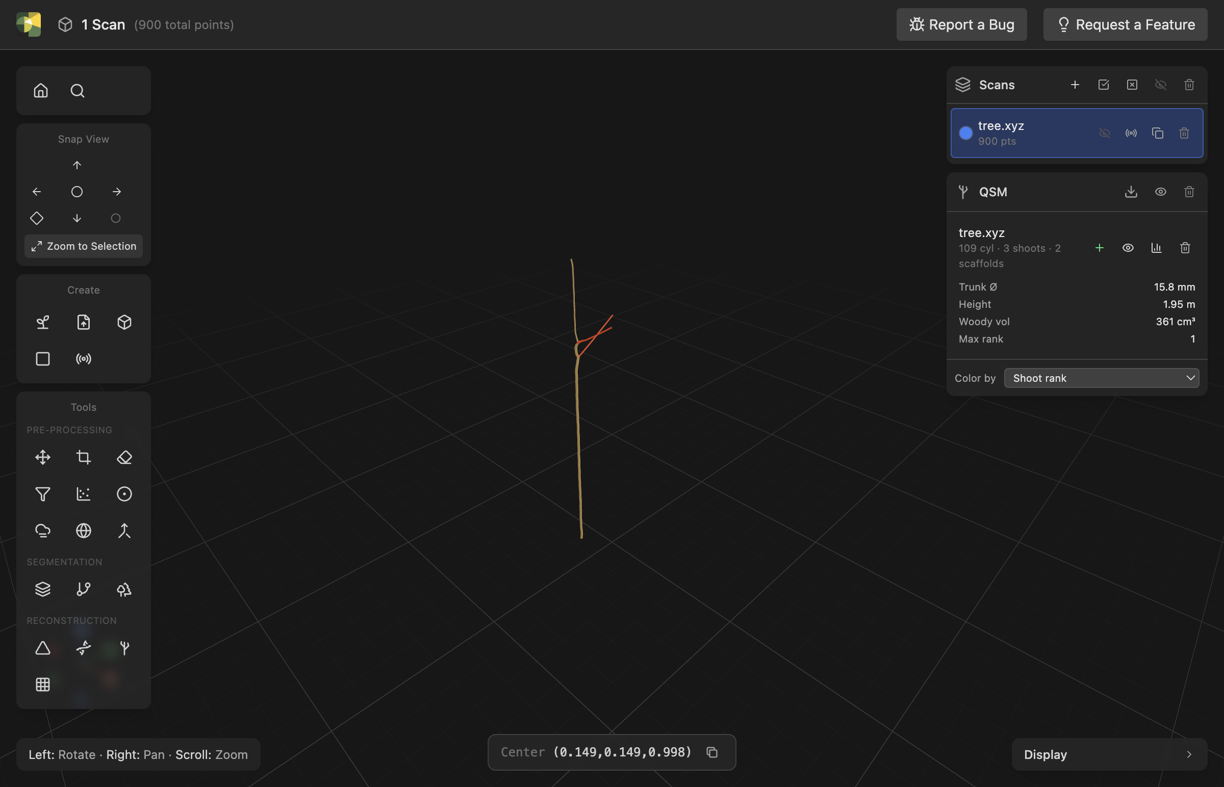
The results panel reports, per QSM:
- Cylinder / shoot / scaffold counts (the row subtitle).
- Trunk Ø — trunk diameter at the base, in mm.
- Height — vertical extent of the woody structure, in m.
- Woody vol — total woody volume, in cm³.
- Max rank — the deepest branching order recovered.
A shoot follows one botanical axis straight through every fork where smaller branches peel off, keeping its rank, rather than restarting at each junction.
View detailed results
For finer-grained analytics on a single tree, click the chart icon ("View results") on the QSM's row. This opens a results window with the per-tree detail that the row's four headline numbers summarize — no re-computation, it reads the model already in memory:
- Scan-coverage badge — an at-a-glance HIGH / MODERATE / LOW grade for how completely the scan saw the woody surface, weighted by volume so the trunk and scaffolds dominate. This is an occlusion diagnostic, not a pass/fail: terrestrial LiDAR only sees one side of each branch, so even an excellent model has modest raw coverage — the build's radius correction is designed to fill in the occluded wood from the taper and pipe-model. A LOW grade means the structure is largely one-sided and the model is inferring more than it measures (add more scan positions), not that the fit is wrong.
- Whole-tree summary — TCSA, trunk diameter, height, canopy extent, total/stem/branch volume, total length, scaffold and shoot counts, plus a reconstructed DBH interpolated from the trunk taper at 1.3 m.
- Stem taper — trunk diameter narrowing with height; one-sided (under-covered) trunk cylinders are tinted amber.
- Branch-order distribution — shoot count, total length, or woody volume per rank (trunk, scaffold, order 2, …).
- Branch-angle distribution — a histogram of each shoot's fork angle against its parent axis (narrow angles flag included-bark risk).
- Scan coverage & fit — a surface-coverage histogram (one-sided bins tinted amber) and an absolute fit-residual (MAD) histogram, shown for information.
- Vertical profile — woody volume (or length) binned by height, reading as a tree silhouette — useful for biomass partitioning.
- Per-shoot table — every shoot with its rank, length, base diameter, fork angle, child count, and volume-weighted surface coverage; click a column header to sort. One-sided shoots are tinted so you can see which parts of the model are inferred rather than measured.
The right column has controls for the branch-angle bin width and the branch-order / vertical-profile metric.
Full per-cylinder geometry for downstream tooling lives in the exported file — see Export below.
Switch the coloring
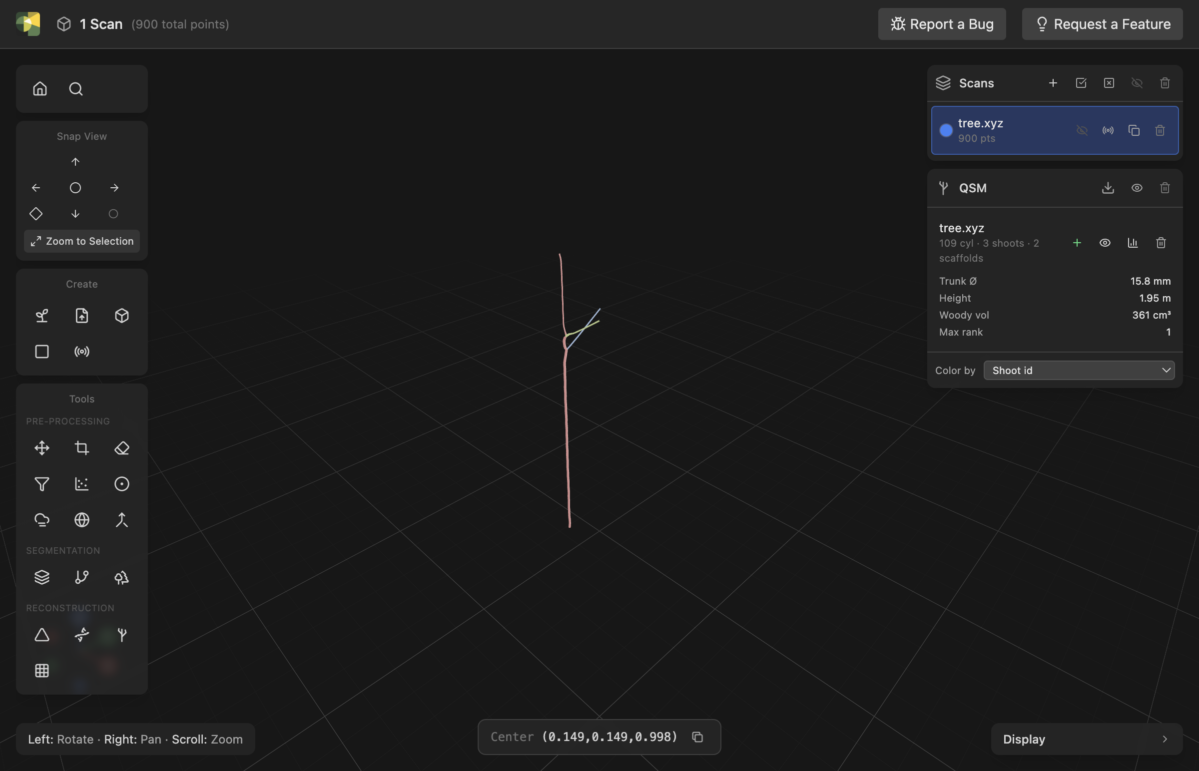
The Color by dropdown at the bottom of the QSM panel offers four modes. The first two encode data as color; the last two are about appearance.
- Shoot rank (default) — colors by branching order: a wood-tan trunk (rank 0), red-orange scaffolds (rank 1), then blue, green, violet, pink for deeper ranks. Best for reading structure.
- Shoot id — gives every shoot its own distinct color, so each continuous axis reads as one object regardless of rank. Best for seeing the shoots themselves.
- Color — one flat color for the whole tree, picked from the swatch or typed as a hex value. Useful for figures where the QSM is context rather than the subject, or to match a house style.
- Texture — wraps a bark image around every branch, for a presentation-ready tree.
Bark textures
In Texture mode two extra controls appear:
- Bark — the bark image. The dropdown lists the five bark textures that ship with the Helios plant-architecture library (almond, apple, grape, olive, western redbud). Upload picks your own JPEG or PNG instead — a photograph of the species you actually scanned, for example. A texture that tiles seamlessly gives the best result.
- Tile (m) — the real-world size of one bark tile, in meters
(default
0.25). Smaller values make the bark pattern finer and repeat more often; larger values make it coarser. This is a physical size, not a repeat count.
Because the tile is defined in world units, the bark stays at a consistent physical scale everywhere on the tree: the pattern on a thick trunk looks the same size as the pattern on a thin branch, instead of being stretched wider as the branch thickens. Only very thin twigs (under a couple of centimeters across) narrow the pattern, where the detail is too small to see anyway.
The bark images are read from the backend, so the first switch into Texture mode may take a moment while the image loads.
See Color modes → QSM for the full palette.
Multi-view scans of one tree
A single tree is often captured from several scanner positions. You have two ways to handle that, shown in the dialog when more than one scan is checked:
| Mode | What it does | Use when |
|---|---|---|
| One QSM from all scans | Fuses the selected scans into a single cloud in world space and builds one QSM | The scans are multiple views of one tree — they must already be aligned (see Register & compare) |
| One QSM per scan | Builds a separate QSM for each selected scan, in sequence | The scans are different trees |
Aggregating multi-view scans gives the most complete model — each scanner position fills in wood the others couldn't see, which directly improves radius accuracy on otherwise one-sided trunks. Align the scans first: the fuse concatenates them in world coordinates and trusts that registration.
Export
A QSM lives in the current viewer session and is not persisted when you close the app — so export it to a file to keep the model, take it into other tooling, or load it again later. Exporting to CSV is the way to keep a QSM: that file imports straight back into Phytograph (see Re-importing a QSM).
- Click the Export (download) icon at the top of the QSM results panel.
- In the export dialog, pick a format, then tick which QSMs to write (all are selected by default — the checkbox next to the list heading toggles them all at once).
- Click Export. For a single QSM you get a save dialog with a suggested filename (the source scan's name, with the format's extension) — edit it to whatever you like before saving. When you selected several QSMs, you choose a folder instead and one file is written per QSM, each named after its source scan.
| Format | What it is | Use it for |
|---|---|---|
| CSV | One row per cylinder — ID, parentID, branchID, branchOrder, segmentID, parentSegmentID, start/end coordinates, axis, radius, length, plus surface-coverage and fit residual. Uses the SimpleForest column layout. |
Keeping the model — this is the only format Phytograph can read back. Also analysis and round-tripping into the standard QSM ecosystem: it follows the SimpleForest schema that rTwig and aRchi read (the TreeQSM-compatible path). The column set is validated against rTwig's importer. |
| OBJ | Triangulated tube mesh with smooth vertex normals — the same geometry the viewport draws. Each shoot is one named object (shoot_<id>_rank_<n>), so the tree arrives separable. Writes a bundle: the .obj, a sibling .mtl, and the bark image in Texture mode. |
Viewing the model anywhere — Blender, CloudCompare, MeshLab, Rhino. |
| PLY | The same tube mesh plus vertex normals, with each face tagged by branch order and radius. | Viewing with attribute-based coloring (color faces by branching order in CloudCompare/Blender). |
Coordinates and units
Exports are in the cloud's world coordinates, in meters. The
CSV root cylinder has parentID = -1.
The mesh exports match the viewport
OBJ and PLY are built from the same geometry the viewer renders: each shoot is swept as one continuous tube, so the surface is seamless and the radius varies smoothly through each joint rather than stepping. There are no end caps — a shoot simply overlaps its parent at the fork, exactly as in the viewport — which also keeps the exported surface area from being inflated by cap faces buried inside the joints.
Consequently the mesh formats carry per-node radii, not one radius per cylinder. If you need the raw fitted cylinder parameters (each with its own single radius, start, and end), export CSV — that's the format that preserves them.
OBJ carries the colors too
The OBJ export writes the color mode you have selected into a sibling
.mtl file, so the tree opens in Blender looking the way it looks in the
viewer rather than as untextured gray. Rank mode writes one material per
rank, Shoot mode one per shoot, Color mode a single material with
your picked color, and Texture mode a bark material plus the bark
image and the UV coordinates that tile it at the size you set.
Keep the exported files together — an .obj separated from its .mtl (and
its images) loses the colors. PLY carries branch_order and radius
per face instead, which is the better choice if you want to color by
branching order in a downstream tool.
Leaves are exported too
If you have added foliage with Add Leaves, the OBJ export
includes it as a final leaves object with its own textured materials, so
the tree opens leafy rather than as a bare winter skeleton. Leaf textures are
alpha cutouts and are exported as such, which is what makes each leaf come
back leaf-shaped instead of as an opaque rectangle.
CSV and PLY carry the woody structure only — leaves are not part of the cylinder model, so re-importing a CSV gives you the bare QSM back and you can re-run Add Leaves on it.
Re-importing a QSM
An exported CSV loads straight back in — drag it onto the window, or use File → Import → QSM CSV…. You get the same model you exported: the same cylinders and shoots, colorable by Shoot rank or Shoot id, and the same trunk diameter, height, woody volume, and max rank in the results panel. (Those metrics aren't stored in the file; they're recomputed from the cylinders.) You can add leaves to a re-imported QSM just as you would a freshly built one.
CSVs written by other SimpleForest/TreeQSM-family tools import too. See Importing a QSM for how Phytograph tells a QSM CSV apart from a point-cloud CSV, and File formats for the columns.
The OBJ and PLY exports are visualization outputs and can't be re-imported as QSMs — they're triangle meshes, with the cylinder topology already baked away. Bringing one back into Phytograph gives you a mesh, not a QSM, so keep the CSV if you want the model itself.
How it works
The QSM pipeline is a clean-room, non-ML, fully deterministic reconstruction (same cloud in → identical model out). It runs five stages; this section explains what each does, the design decisions behind them, and the hard-coded parameters you can't see in the UI.
The five stages
-
Skeleton (geodesic level-set). A neighbor graph is built over the points (a k-d tree radius graph), true geodesic distance from the tree base (the lowest points of the graph's largest connected component, so stray debris below the tree can't become the root) is computed with Dijkstra, and points are binned into level sets by that distance. Each connected component in a level becomes one skeleton node; adjacent levels are linked into a rooted, acyclic tree. Occlusion gaps that would disconnect the crown are bridged so the geodesic field still reaches it. This is deterministic by construction — no iterative contraction, no RNG.
-
Shoot segmentation + rank (the headline). The skeleton is collapsed into segments (chains between forks). Each segment's GrowthLength — its own length plus everything it supports distally — is computed in one pass. At every fork, the continuation child is the one with the largest GrowthLength; it inherits the parent's shoot and rank, while every other child starts a new shoot at rank + 1. A shoot is then a maximal chain of continuation-linked segments, and its rank is the number of forks between it and the base.
Why largest-subtree, not thickest or straightest?
The continuation rule decides which way an axis "keeps going." Phytograph uses the largest-GrowthLength child (the rule used by aRchi and SimpleForest) because it is the most robust under noisy radii and angle jitter — a thicker or straighter sibling will not steal the leader. The rule is actually a weighted score
w_L·GrowthLength + w_A·CrossSection + w_θ·colinearity, but the validated default weights are(1, 0, 0)— pure largest-subtree. -
Cylinder fitting. Each cloud point is assigned to the cylinder whose axis is nearest (a global nearest-cylinder competition, so a branch keeps its own bark instead of being absorbed by the trunk), and a robust least-squares cylinder is fit to each cylinder's points. The fit is a deterministic Huber/IRLS M-estimator (not RANSAC). Each cylinder also gets two quality numbers: surface coverage (
surf_cov— what fraction of its surface the scanner actually saw; low means one-sided/occluded) and mad (mean fit residual). -
Radius correction. Raw per-cylinder fits are locally noisy and, on occluded wood, biased. This stage turns them into a coherent radius field with four principled ingredients:
- Per-shoot monotone taper — a shoot's radius must shrink from base to tip. An isotonic (PAVA) fit, weighted by surface coverage, forces that. The taper is keyed to distance from the base, not GrowthLength (GrowthLength drops at every fork, which used to make a still-thick trunk go thin right after a big branch).
- Pipe-model lower bound — a parent must be at least as fat as the wood it carries, propagated tip→base. This keeps a heavily occluded trunk thick by construction from the branches it supports, instead of collapsing to the minimum radius.
- Twig anchor — leaf cylinders are floored at the twig radius you set, so tips don't taper to zero.
- Cross-fork cap — a child branch cannot be fatter than the parent it grows from. Applied last, this caps any child-shoot base that still exceeds its parent at the junction (a sparse one-sided arc can otherwise balloon a thin branch's base fit). It only ever lowers the child, so a thin parent fit can never cascade outward.
The correction only changes radius — topology, shoots, and ranks are never touched.
-
Metrics. The horticultural summary you see in the results panel — TCSA, trunk diameter, height, scaffold count, per-rank length / diameter / crotch angle, and woody volume split into stem vs. branch.
Hard-coded parameters
Everything except twig radius and axis continuation (and the hidden continuation weights) is fixed at a validated default. The most relevant:
| Parameter | Value | What it controls |
|---|---|---|
| Min points to build | 50 | Below this the build refuses |
| Point cap | 60,000 | Clouds are downsampled to this before building |
| Backend hard cap | 3,000,000 | A backstop for callers that bypass the downsample (scripted / direct API use); the build refuses rather than running for minutes |
| Twig radius (UI) | 4.23 mm | Tip diameter the taper is anchored to |
| Continuation weights | (1, 0, 0) | Largest-GrowthLength axis rule |
| Axis continuation (UI) | 0.75 | Sibling-thickness ratio at/above which a fork is codominant and the shoot ENDS there |
| Fork size floor | 0.50 | Both arms must carry comparable distal length before a fork can end an axis |
| Structural floors | 1% of tree length, 0.35 x trunk radius | Keep crown twigs from ending an axis (they fork symmetrically too) |
| Short-branch prune | 0.10 m | Leaf fragments shorter than this are dropped as skeleton noise |
| Cylinder fit | Huber IRLS, k = 1.345 | Robust M-estimator (no RANSAC) |
| Point→cylinder cutoff | 0.5 m | Points farther than this from any axis are ignored (other trees, ground) |
| Surface-coverage trust | 0.7 | At/above this a fitted radius is trusted; below it leans on the taper / pipe-model |
| Pipe-model exponent | 2.5 | r_parent ≥ (Σ r_child^k)^(1/k) — slightly above area conservation |
Known limitations
These are honest, validated behaviors — not bugs:
- Determinate trunks (a short trunk ending in a whorl of scaffolds): the largest-subtree rule can carry rank 0 a little way up one scaffold, so the "trunk" shoot slightly over-extends. The trade-off is deliberate — tightening it would lose real scaffolds. Central-leader trees (a trunk that genuinely continues to the apex) are tracked perfectly.
- The finest twigs can merge into their parent where the skeleton's resolution runs out. Total branch length is still recovered even when the tip count is low.
- Branch radius under heavy occlusion is reported with more uncertainty than the trunk; this is why woody volume is split into stem vs. branch — the stem number is the trustworthy one.
Common problems
"No cylinders could be fitted: the skeleton reached only N of M points." The skeleton couldn't connect the crown to the base. Make sure the ground is removed but the trunk base is intact, and that the cloud isn't so decimated that branches are disconnected. Aggregating multiple scan positions helps. A few stray points left over from ground removal are fine: the skeleton roots at the lowest points of the largest connected piece of the cloud, so small detached patches below or beside the tree are ignored.
"The trunk radius looks too thin / too thick." On a one-sided scan the trunk's own points are unreliable; the model leans on the pipe-model from the branches it carries. More scan coverage (aggregate multiple views) is the real fix. The trunk diameter the panel reports is measured at the base.
"A scaffold got colored like the trunk (rank 0)." That's the determinate-trunk limitation above — the leader continued up a scaffold. Switch to Shoot id coloring to see the actual shoot boundaries.
What's next
- Add leaves to the QSM to build a foliated reconstruction from the woody model.
- Compare the QSM's metrics to a generated plant model of the same species.
- Read the QSM concept page for how cylinders, shoots, and ranks relate to skeletons and meshes.